Taichi - Physics Engines
Games 201 - ADVANCED PHYSICS ENGINES
Lecturer: Dr. Yuanming Hu
Taichi Graphics Course S1 (for completion and new feature updates)
Lecturer: Dr. Tiantian Liu
Some supplement contents about Taichi
If overlapping contents: just add on the original GAMES201 notes. The new contents: add at the last of the notes individually.
- Exporting Results (Lecture 2)
- OOP and Metaprogramming (Lecture 3)
- Diff. Programming (Lecture 3)
- Visualization (Lecture 3)
Lecture 1 Introduction
Keyword: Discretization / Efficient solvers / Productivity / Performance / Hardware architecture / Data structures / Parallelization / Differentiability (DiffTaichi)
Taichi Programming Language
Initialization
Required every time using taichi
Use ti.init, for spec. cpu or gpu: use ti.cpu (default) or ti.gpu
ti.init(arch=ti.cuda) # spec run in any hardwareData
Data Types
signed integers ti.i8 (~ 64, default i32) / unsigned integers ti.u8 (~64) / float-point numbers ti.f32(default) (~ 64)
Modify Default
The default can be changed via ti.init
ti.init(default_fp=ti.f32)ti.init(default_ip=ti.i64)
Type Promotions
- i32 + f32 = f32
- i32 + i64 = i64
Switch to high percision automatically
Type Casts
Implicit casts: Static types within the Taichi Scope
xxxxxxxxxxdef foo(): # Directly inside Python scopea = 1a = 2.7 # Python can re-def types automaticallyprint(a) # 2.7xxxxxxxxxx.kernel # Inside Taichi scopedef foo():a = 1 # already def as a int typea = 2.7 # re-def failed (in Taichi)print(a) # 2Explicit casts:
variable = ti.casts(variable, type)xxxxxxxxxx.kerneldef foo():a = 1.8b = ti.cast(a, ti.i32) # switch to int; b = 1c = ti.cast(b, ti.f32) # switch to floating; c = 1.0
Tensor
Multi-dimensional arrays(高维数组)
Self-defines: Use
ti.typesto create compound types including vector / matrix / structximport taichi as titi.init(arch = ti.cpu)# Define your own types of datavec3f = ti.types.vector(3, ti.f32) # 3-dimmat2f = ti.types.matrix(2, 2, ti.f32) # 2x2ray = ti.types.struct(ro = vec3f, rd = vec3f, l = ti.f32).kerneldef foo():a = vec3f(0.0)print(a) # [0.0, 0.0, 0.0]d = vec3f(0.0, 1.0, 0.0)print(d) # [0.0, 1.0, 0.0]B = mat2f([[1.5, 1.4], [1.3, 1.2]])print("B = ", B) # B = [[1.5, 1.4], [1.3, 1.2]]r = ray(ro = a, rd = d, l = 1)print("r.ro = ", r.ro) # r.ro = [0.0, 0.0, 0.0]print("r.rd = ", r.rd) # r.rd = [0.0, 1.0, 0.0]foo()Pre-defines: An element of the tensors can be either a scalar (
var), a vector (ti.Vector) or a matrix (ti.Matrix) (ti.Struct)Accessed via
a[i, j, k]syntax (no pointers)xxxxxxxxxximport taichi as titi.init()a = ti.var(dt=ti.f32, shape=(42, 63)) # A tensor of 42x63 scalarsb = ti.Vector(3, dt=ti.f32, shape=4) # A tensor of 4x 3D vectors (3 - elements in the vector, shape - shape of the tensor, composed by 4 3D vectors)C = ti.Matrix(2, 2, dt=ti.f32, shape=(3, 5)) # A tensor of 3x5 2x2 matricesloss = ti.var(dt=ti.f32, shape=()) # A 0-D tensor of a single scalar (1 element)a[3, 4] = 1print('a[3, 4] = ', a[3, 4]) # a[3, 4] = 1.000000b[2] = [6, 7, 8]print('b[0] =', b[0][0], b[0][1], b[0][2]) # b[0] not yet supported (working)loss[None] = 3print(loss[None]) # 3
Field
ti.field: A global N-d array of elements
heat_field = ti.field(dtype=ti.f32, shape=(256, 256))
global: a field can be read / written from both Taichi scope and Python scope
N-d: Scalar (N = 0); Vector (N = 1); Matrix (N = 2); Tensor (N = 3, 4, 5, …)
elements: scalar, vector, matrix, struct
access elements in a field using [i, j, k, …] indexing
xxxxxxxxxximport taichi as titi.init(arch=ti.cpu)pixels = ti.field(dtype=float, shape=(16, 8))pixels[1,2] = 42.0 # index the (1,2) pixel on the screenxxxxxxxxxximport taichi as titi.init(arch=ti.cpu)vf = ti.Vector.field(3, ti.f32, shape=4) # 4x1 vectors, every vector is 3x1.kerneldef foo():v = ti.Vector([1, 2, 3])vf[0] = vSpecial Case: access a 0-D field using
[None]xxxxxxxxxxzero_d_scalar = ti.field(ti.f32, shape=())zero_d_scalar[None] = 1.5 # Scalar in the scalar fieldzero_d_vector = ti.Vector.field(2, ti.f32, shape=())zero_d_vector[None] = ti.Vector([2.5, 2.6])
Other Examples:
3D gravitational field in a 256x256x128 room
gravitational_field = ti.Vector.field(n=3, dtype=ti.f32, shape=(256, 256, 128))2D strain-tensor field in a 64x64 grid
strain_tensor_field = ti.Matrix.field(n = 2, m = 2, dtype = ti.f32, shape = (64, 64))a global scalar that want to access in a taichi kernel
global_scalar = ti.field(dtype = ti.f32, shape=())
Kernels
Must be decorated with @ti.kernel (Compiled, statically-typed, lexically-scoped, parallel and differentiable - faster)
For loops at the outermost scope in a Taichi kernel is automatically parallelized (if inside - serial)
If a outermost scope is not wanted to parallelize for and an inside scope is, write the unwanted one in the python scope and call the other one as the outermost in the kernel.
Arguments
At most 8 parameters
Pass from Python scope to the Taichi scope
Must be type-hinted
xxxxxxxxxx.kerneldef my_kernel(x: ti.i32, y: ti.f32): # explicit input variables with typesprint(x + y)my_kernel(2, 3.3) # 5.3Scalar only (if vector needs to input separately)
Pass by value
Actually copied from the var. in the Python scope and if the values of some var.
xis modified in the Taichi kernel, it won’t change in the Python scope.
Return Value
May or may not return
Returns one single scalar value only
Must be type-hinted
xxxxxxxxxx.kerneldef my_kernel() -> ti.i32: # returns i32return 233.666print(my_kernel()) # 233 (casted to int32)
Functions
Decorated with @ti.func, usually for high freq. used func.
Taichi's function can be called in taichi's kernel but can't be called by python (not global)
Function 可以被 kernel 调用但不能被 py 调用,kernel 也不能调用 kernel,但是 function可以调用 function
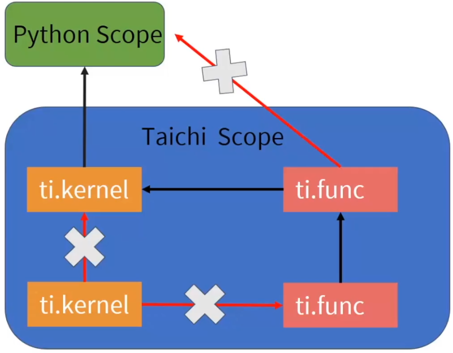
- Taichi functions can be nested (function in function)
- Taichi functions are force-inlined (cannot iterate)
Arguments
Don’t need to be type-hinted
Pass by value (for the force-inlined
@ti.func)if want to pass outside, use
return
Scalar Math
Similar to python. But Taichi also support chaining comparisons (a < b <= c != d)
Specifically, a / b outputs floating point numbers, a // b ouputs integer number (as in py3)
Matrices and Linear Algebra
ti.Matrix is for small matrices only. For large matrices, 2D tensor of scalars should be considered.
Note that element-wise product in taichi is * and mathematically defined matrix product is @ (like MATLAB)
Common Operations:(返回矩阵 A 经过变换的结果而非变换 A 本身)
xxxxxxxxxxA.transpose() # 转置A.inverse() # 逆矩阵A.trace() # 迹A.determinant(type)A.normalized() # 向量除以自己模长A.norm() # 返回向量长度A.cast(type) # 转换为其他数据类型ti.sin(A)/cos(A) # element wise(给 A 中所有元素都做 sin 或者 cos 运算)Parallel for-loops
(Automatically parallalized)
Range-for loops
Same as python for loops
Struct-for loops
Iterates over (sparse) tensor elements. Only lives at the outermost scope looping over a ti.field
for i,j in x: can be used
Example:
xxxxxxxxxximport taichi as ti
ti.init(arch=ti.gpu) # initiallize every time
n = 320pixels = ti.var(dt=ti.f32, shape=(n*2, n)) # every element in this tensor is 32 bit float point number,shape 640x320
.kerneldef paint(t: ti.f32): for i, j in pixels: # parallized over all pixel pixels[i, j] = i * 0.001 + j * 0.002 + t # This struct-for loops iterate over all tensor coordinates. i.e. (0,0), (0,1), (0,2), ..., (0,319), (1,0), ..., (639,319) # Loop for all elements in the tensor # For this dense tensor, every element is active. But for sparse tensor, struct-for loop will only work for active elementspaint(0.3)breakis NOT supported in the parallel for-loops
Atomic Operations
In Taichi, augmented assignments (e.g. x[i] += 1) are automatically atomic.
(+=: the value on the RHS is directly summed on the current value of the var. and the referncing var.(array))
(Atomic operation: an operation that will always be executed without any other process being able to read or change state that is read or changed during the operation. It is effectively executed as a single step, and is an important quality in a number of algorithms that deal with multiple independent processes, both in synchronization and algorithms that update shared data without requiring synchronization.)
When modifying global var. in parallel, make sure to use atomic operations.
xxxxxxxxxx.kerneldef sum(): # to sum up all elements in x for i in x: # Approach 1: OK total[None] += x[i] # total: 0-D tensor => total[None] # Approach 2: OK ti.atomic_add(total[None], x[i]) # will return value before the atomic addition # Approach 3: Wrong Result (Not atomic) total[None] = total[None] + x[i] # other thread may have summedTaichi-scope vs. Python-scope
Taichi-scope: Everything decorated with ti.kernel and ti.func
Code in Taichi-scope will be compiled by the Taichi compiler and run on parallel devices (Attention that in parallel devices the order of print may not be guaranteed)
Static data type in the Taichi scope
The type won’t change even if actually defines some other values / fields (error)
Static lexical scope in the Taichi scope
xxxxxxxxxx.kerneldef err_out_of_scope(x:float):if x < 0: # abs value of xy = -xelse:y = xprint(y) # y generated in the 'if' and not pass outside, error occursCompiled JIT (just in time) (cannot see Python scope var. at run time)
xxxxxxxxxxa = 42.kerneldef print_a():print('a = ', a)print_a() # 'a = 42'a = 53print('a = ', a) # 'a = 53'print_a() # still 'a = 42'Another demo:
xxxxxxxxxxd = 1.kerneldef foo():print('d in Taichi scope = ', d)d += 1 # d = 2foo() # d in Taichi scope = 2 (but after this call, ti kernel will regard d as a constant)d += 1 # d = 3foo() # d in Taichi scope = 2 (d not changed in Ti-scope but changed in Py-scope)If want real global: use
ti.fieldxxxxxxxxxxa = ti.field(ti.i32, shape=()).kerneldef print_a():print('a=', a[None])a[None] = 42print_a() # "a= 42"a[None] = 53print_a() # "a= 53"
Python-scope: Code outside the Taichi-scope
Code in Python-scope is simple py code and will be executed by the py interpreter
Phases
Initialization:
ti.init()Tensor allocation:
ti.var,ti.Vector,ti.MatrixOnly define tensors in this allocation phase and never define in the computation phase
Computation (launch kernel, access tensors in Py-scope)
Optional: Restart (clear memory, destory var. and kernels):
ti.reset()
Practical Example (fractal)
xxxxxxxxxximport taichi as ti
ti.init(arch=ti.gpu)
n = 320pixels = ti.var(dt=ti.f32, shape=(n * 2, n))
.funcdef complex_sqr(z): return ti.Vector([z[0]**2 - z[1]**2, z[1] * z[0] * 2]) # calculate the square of a complex number # In this example, use a list and put in [] to give values for ti.Vector
.kerneldef paint(t: ti.f32): # time t - float point 32 bit for i, j in pixels: # parallized over all pixels c = ti.Vector([-0.8, ti.cos(t) * 0.2]) z = ti.Vector([i / n - 1, j / n - 0.5]) * 2 # Julia set formula iterations = 0 # iterate for all pixels while z.norm() < 20 and iterations < 50: z = complex_sqr(z) + c # user-defined in @ti.func iterations += 1 pixels[i, j] = 1 - iterations * 0.02 gui = ti.GUI("Julia Set", res = (n*2, n)) # ti's gui
for i in range(1000000): paint(i * 0.03) gui.set_image(pixels) gui.showDebug Mode
Lecture 2 Lagrangian View
Two Views (Def)
Lagrangian View
Sensors that move passively with the simulated material(节点跟随介质移动)
粒子会被额外记录位置,会随(被模拟的)介质不断移动
Euler View
Still sensors that never moves(穿过的介质的速度)
网格中每个点的位置不会被特别记录
Mass-Spring Systems
弹簧 - 质点模型 (Cloth / Elastic objects / ...)
Hooke's Law
(f - force, k - Spring stifness, Li,j - Spring rest length between particle i and j, ^ - normalization,
Newton's Second Law of Motion
Time Integration
Common Types of Integrators
Forward Euler (explict)
Semi-implicit Euler (aka. Symplectic Euler, Explicit)
(准确性上提升,以
Backward Euler (often with Newton's Method, Implicit)
Full implement see later
Comparison
Explicit: (forward Euler / symplectic Euler / RK (2, 3, 4) / ...)
Future depends only on past, easy to implement, easy to explode, bad for stiff materials
~ 数值稳定性,不会衰减而是随时间指数增长
Implicit (back Euler / middle-point)
Future depends on both future and past, harder to implement, need to solve a syustem of (linear) equation, hard to optimize, time steps become more expensive but time steps are larger, extra numerical damping and locking (overdamping) (but generally, uncoonditionally stable)
(显式 - 容易实现,数值上较为不稳定,受 dt 步长影响较大;隐式 - 难实现,允许较长步长)
Implementing a Mass-Spring System with Symplectic Euler
Steps
- Compute new velocity using
- Collision with ground
- Compute new position using
Demo
xxxxxxxxxximport taichi as ti
ti.init(debug=True)
max_num_particles = 256
dt = 1e-3
num_particles = ti.var(ti.i32, shape=())spring_stiffness = ti.var(ti.f32, shape=())paused = ti.var(ti.i32, shape=())damping = ti.var(ti.f32, shape=())
particle_mass = 1bottom_y = 0.05
x = ti.Vector(2, dt=ti.f32, shape=max_num_particles)v = ti.Vector(2, dt=ti.f32, shape=max_num_particles)
A = ti.Matrix(2, 2, dt=ti.f32, shape=(max_num_particles, max_num_particles))b = ti.Vector(2, dt=ti.f32, shape=max_num_particles)
# rest_length[i, j] = 0 means i and j are not connectedrest_length = ti.var(ti.f32, shape=(max_num_particles, max_num_particles))
connection_radius = 0.15
gravity = [0, -9.8]
.kerneldef substep(): # 每一个新的时间步,把每一帧分为若干步(在模拟中 time_step 需要取相应较小的数值) # Compute force and new velocity n = num_particles[None] for i in range(n): # 枚举全部 i v[i] *= ti.exp(-dt * damping[None]) # damping total_force = ti.Vector(gravity) * particle_mass # 总受力 G = mg for j in range(n): # 枚举其余所有粒子 是否有关系 if rest_length[i, j] != 0: # 两粒子之间有弹簧? x_ij = x[i] - x[j] total_force += -spring_stiffness[None] * (x_ij.norm() - rest_length[i, j]) * x_ij.normalized() # 胡克定律公式 -k * ((xi - xj).norm - rest_length) * (xi - xj).norm v[i] += dt * total_force / particle_mass # sympletic euler: 用力更新一次速度 # Collide with ground (计算完力和速度之后立刻与地面进行一次碰撞) for i in range(n): if x[i].y < bottom_y: # 一旦发现有陷入地下的趋势就把速度的 y component 设置为 0 x[i].y = bottom_y v[i].y = 0
# Compute new position for i in range(num_particles[None]): x[i] += v[i] * dt # 新的位置的更新:把速度产生的位移累加到位置上去
.kerneldef new_particle(pos_x: ti.f32, pos_y: ti.f32): # Taichi doesn't support using Matrices as kernel arguments yet new_particle_id = num_particles[None] x[new_particle_id] = [pos_x, pos_y] v[new_particle_id] = [0, 0] num_particles[None] += 1 # Connect with existing particles for i in range(new_particle_id): dist = (x[new_particle_id] - x[i]).norm() if dist < connection_radius: rest_length[i, new_particle_id] = 0.1 rest_length[new_particle_id, i] = 0.1 gui = ti.GUI('Mass Spring System', res=(512, 512), background_color=0xdddddd)
spring_stiffness[None] = 10000damping[None] = 20
new_particle(0.3, 0.3)new_particle(0.3, 0.4)new_particle(0.4, 0.4)
while True: for e in gui.get_events(ti.GUI.PRESS): if e.key in [ti.GUI.ESCAPE, ti.GUI.EXIT]: exit() elif e.key == gui.SPACE: paused[None] = not paused[None] elif e.key == ti.GUI.LMB: new_particle(e.pos[0], e.pos[1]) elif e.key == 'c': num_particles[None] = 0 rest_length.fill(0) elif e.key == 's': if gui.is_pressed('Shift'): spring_stiffness[None] /= 1.1 else: spring_stiffness[None] *= 1.1 elif e.key == 'd': if gui.is_pressed('Shift'): damping[None] /= 1.1 else: damping[None] *= 1.1 if not paused[None]: for step in range(10): substep() X = x.to_numpy() gui.circles(X[:num_particles[None]], color=0xffaa77, radius=5) gui.line(begin=(0.0, bottom_y), end=(1.0, bottom_y), color=0x0, radius=1) for i in range(num_particles[None]): for j in range(i + 1, num_particles[None]): if rest_length[i, j] != 0: gui.line(begin=X[i], end=X[j], radius=2, color=0x445566) gui.text(content=f'C: clear all; Space: pause', pos=(0, 0.95), color=0x0) gui.text(content=f'S: Spring stiffness {spring_stiffness[None]:.1f}', pos=(0, 0.9), color=0x0) gui.text(content=f'D: damping {damping[None]:.2f}', pos=(0, 0.85), color=0x0) gui.show()Backward Euler Implicit Implement
Steps
- Eliminate
- Linearize (Newton's):
- Clean up:
- To solve the equation: Jacobi / Gauss-Seidel iteration OR conjugate gradients
Solving the system:
Demo
xxxxxxxxxximport taichi as tiimport random
ti.init()
n = 20
A = ti.var(dt=ti.f32, shape=(n, n)) # 20 x 20 Matrixx = ti.var(dt=ti.f32, shape=n)new_x = ti.var(dt=ti.f32, shape=n)b = ti.var(dt=ti.f32, shape=n)
.kernel # iteration kerneldef iterate(): for i in range(n): r = b[i] for j in range(n): if i != j: r -= A[i, j] * x[j] new_x[i] = r / A[i, i] # 每次都更新 x 使得 x 能满足矩阵一行或一个的线性方程组(局部更新)- 对性质好的矩阵逐渐收敛 for i in range(n): x[i] = new_x[i]
.kernel # Compute residual b - A * xdef residual() -> ti.f32: # residual 一开始会非常大 经过若干次迭代会降到非常低 res = 0.0 for i in range(n): r = b[i] * 1.0 for j in range(n): r -= A[i, j] * x[j] res += r * r return res
for i in range(n): # 初始化矩阵 for j in range(n): A[i, j] = random.random() - 0.5
A[i, i] += n * 0.1 b[i] = random.random() * 100
for i in range(100): # 执行迭代 iterate() print(f'iter {i}, residual={residual():0.10f}')
for i in range(n): lhs = 0.0 for j in range(n): lhs += A[i, j] * x[j] assert abs(lhs - b[i]) < 1e-4Unifying Explicit and Implicit Integrators
Solve Faster
For millions of mass points and springs
- Sparse Matrices
- Conjugate Gradients
- Preconditioning
- Use Position-based Dynamics
Lagrangian Fluid Simulation (SPH)
Smoothed Particle Hydrodynamics
Use particles carrying samples of physical quntities, and a kernel
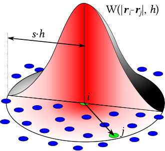
在 x 这点的物理场的值(即
不需要 mesh,适合模拟自由表面 free-surface flows 流体(如水和空气接触的表面,反之,不适合烟雾(空间需要被填满)等),可以使用 “每个粒子就是以小包水” 理解
Equation of States (EOS)
aka. Weakly Compressible SPH (WCSPH)
Momentum Equation (
(Actually the Navier-Stoke's without considering viscosity)
Gradient in SPH
Not really accurate but at least symmetric and momentum conserving (to add viscosity etc. Laplacian should be introduced)
SPH Simulation Cycle
For each particle
For each particle
Symplectic Euler steps (similar as the mass-spring model)
Variant of SPH
- Predictive-Corrective Impcompressible SPH (PCI-SPH) - 无散,更接近不可压缩
- Position-based Fluids (PBF) (Demo:
ti eample pbf2d) - Position-based dynamics + SPH - Divergence-free SPH (DFSPH) - (velocity)
Paper: SPH Fluids in Computer Graphics, Smooted Particle Hydrodynamics Techniques for Physics Based Simulation of Fluids and Solids (2019)
Courant-Friedrichs-Lewy (CFL) Conditions (Explicit)
One upper bound of time step size: (def. using velocity other than stiffness)
(
Application: estimating allowed time step in (explicit) time integration.
SPH: ~ 0.4; MPM (Material Point Method): 0.3 ~ 1; FLIP fluid (smoke): 1 ~ 5+
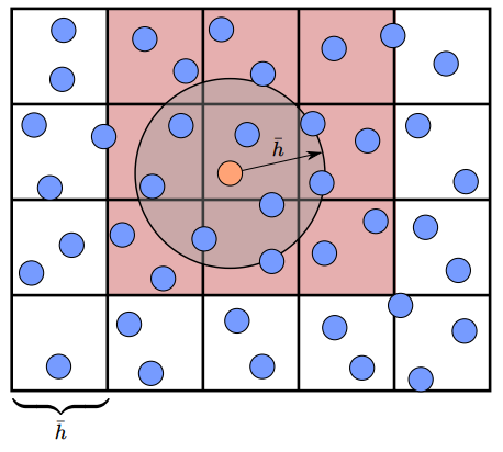
Accelerating SPH: Neighborhood Search
Build spatial data structure such as voxel grids
Neighborhood search with hashing
精确找到距离不超过
Ref: Compact hashing
Other Paricle-based Simulation Methods
- Discrete Element Method (DEM) - 刚体小球,如沙子模拟
- Moving Particle Semi-implicit (MPS) - 增强 fluid incompressibility
- Power Particles - Incompressible fluid solver based on power diagrams
- A peridynamics perspective on spring-mass fracture
Exporting Results
Exporting Videos
ti.GUI.show: save screenshots /ti.imwrite(img, filename)ti video: createsvideo.mp4(-f 24/-f 60)ti gif -i input.mp4: Convertmp4togif
Lecture 3 Lagrangian View (2)
弹性、有限元基础、Taichi 高级特性
Elasticity
Deformation
Deformation Map
Deformation gradient
Deform / rest volume ratio: F[None] = [[2, 0], [0, 1]](横向拉伸了))
Elasticity
Hyperelastic material
Hyperelastic material: Stress-strain relationship is defined by a strain energy density function
Stress Tensor
- The First Piola-Kirchhoff stress tensor (PK1):
- Kirchhoff stress:
- Cauchy stress tensor:
Relationship:
Elastic Moduli (Isotropic Materials)
- Young’s Modulus:
- Bulk Modulus:
- Poisson’s Ratio:
Lame parameters
- Lame’s first parameter:
- Lame’s second parameter (shear modulus /
Conversions:(通常指定 Young’s Modulus & Poisson’s Ratio,或
Hyperelastic Material Models
Popular in graphics:
Linear elasticity (small deformation only, not consistence in rotation) - linear equation systems
Neo-Hookean: (Commonly used in isotropic materials)
(Fixed) Corotated:
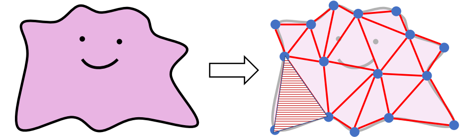
Lagrangian Finite Elements on Linear Tetrahedral Meshes
The Finite Element Method (FEM)
Discretization sheme to build discrete equations using weak formulations of continuous PDEs
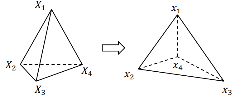
Linear Tetrahedral (Triangular) FEM
Assumption: The deformation map
For every element
Computing
Vertices:
Eliminate
Explicit Linear Triangular (FEM) Simulation
Semi-implicit Euler time integration scheme:
Taichi’s AutoDiff system can use to compute
xxxxxxxxxxfor s in range(30): with ti.Tape(total_energy): # Automatically diff. and write into a 'tape' and use in semi-implicit EulerImplicit Linear Triangular FEM Simulation
Backward Euler Time Integration:
(
Compute force differentials:
Higher Level of Taichi
Objective Data-Oriented Programming
OOP -> Extensibility / Maintainability
An “object” contains its own data (py-var. / ti.field) and method (py-func. / @ti.func / @ti.kernel)

Python OOP in a Nutshell
xxxxxxxxxxclass Wheel: # def a class of 'wheel' def __init__(self, radius, width, rolling_fric): # data, for a wheel: radius / width / fric self.radius = radius # convert all data as `self.` (inside member of 'self') self.width = width self.rolling_fric = rolling_fric def Roll(self): # Method of the 'wheel' ... w1 = Wheel(5, 1, 0.1) # Instantiated Objects (different wheels)w2 = Wheel(5, 1, 0.1)w3 = Wheel(6, 1.2, 0.15)w4 = Wheel(6, 1.2, 0.15)If want to add some features, this method can inherit all past features and add on them (easy to maintain and extent)
Using Classes in Taichi
Hybrid scheme: Objective Data-Oriented Programming (ODOP)
-> More data-oriented -> usually use more vectors / matrices in the class
Important Decorators:
@ti.data_orientedto decorateclass@ti.kernelto decorate class members functions that are Taichi kernels@ti.functo decorate class members functions that are Taichi functions
Caution: if the variable is passed from Python scope, the self.xxx will still regard as a constant
Features:
- Encapsulation: Different classes can be stored in various
.pyscripts and can be called usingfrom [filename] import [classname]in themainscript. - Inheritance: A @data_oriented class can inherit from another @data_oriented class. Both the data and methods are inherited from the base class.
- Polymorphism: Define methods in the child class that have the same name as the methods in the parent class. Proper methods will be called according to the instantiated objects.
Demo: ti example odop_solar:
xxxxxxxxxximport taichi as ti
.data_orientedclass SolarSystem: def __init__(self, n, dt): # n - planet number; dt - time step size self.n = n self.dt = dt self.x = ti.Vector(2, dt=ti.f32, shape=n) self.v = ti.Vector(2, dt=ti.f32, shape=n) self.center = ti.Vector(2, dt=ti.f32, shape=()) # @ti.func 还可以被额外的 @staticmethod(静态函数,同 py)修饰 .func # 生成一个随机数 def random_around(center, radius): # random number in [center - radius, center + radius] return center + radius * (ti.random() - 0.5) * 2 .kernel def initialize(self): # initialize all the tensors for i in range (self.n): offset = ti.Vector([0.0, self.random_around(0.3, 0.15)]) self.x[i] = self.center[None] + offset self.v[i] = [-offset[1], offset[0]] self.v[i] *= 1.5 / offset.norm() .func # still in class def gravity(self, pos): offset = -(pos - self.center[None]) return offset / offset.norm()**3 .kernel # sympletic Euler def integrate(self): for i in range(self.n): self.v[i] += self.dt * self.gravity(self.x[i]) self.x[i] += self.dt * self.v[i] solar = SolarSystem(9, 0.0005) # 9 for n (planet number); 0.0005 for dtsolar.center[None] = [0.5, 0.5]solar.initialize()
gui = ti.GUI("Solar System", background_color = 0x25A6D9)
while True: if gui.get_event(): if gui.event.key == gui.SPACE and gui.event.type == gui.PRESS: solar.initialize() for i in range(10): solar.integrate() gui.circle([0.5, 0.5], radius = 20, color = 0x8C274C) gui.circles(solar.x.to_numpy(), radius = 5, color = 0xFFFFFF) gui.show()Metaprogramming 元编程
Allow to pass almost anything (including tensors) to Taichi kernels; Improve run-time performance by moving run-time costs to compile time; Achieve dimensionality independence (2D / 3D simulation codes simultaneously); etc. 很多计算可以在编译时间完成而非运行时间完成 (kernels are lazily instantiated)
Metaprogramming -> Reusability:
Programming technique to generate other programs as the program’s data

In Taichi the “Codes to write” section is actually ti.templates and ti.statics
Template
Allow to pass anything supported by Taichi (if directly pass something like a = [43, 3.14] (python list) -> error; need to modify as Taichi’s types a = ti.Vector([43, 3.14]))
- Primary types:
ti.f32,ti.i32,ti.f64 - Compound Taichi types:
ti.Vector(),ti.Matrix() - Taichi fields:
ti.field(),ti.Vector.field(),ti.Matrix.field(),ti.Struct.field() - Taichi classes:
@ti.data_oriented
Taichi kernels are instantiated whenever seeing a new parameter (even same typed)
frequently used of templates will cause higher time costs
xxxxxxxxxx.kernel# when calling this kernel, pass these 2 1D tensors (x, y) into template arguments (better to have same magnitude)def copy(x: ti.template(), y: ti.template(), c: ti.f32): # template => to deliver fields for i in x: y[i] = x[i] + c # OK if the shape is the same (regardless the size)Pass-by-reference:
- Computations in the Taichi scope can NOT modify Python scope data (field is global, OK to modify)
- Computations in the Taichi scope can modify Taichi scope data (stored in the same RAM location)
xxxxxxxxxxvec = ti.Vector([0.0, 0.0])
.kerneldef my_kernel(x: ti.template()): # x[0] = 2.0 is bad assignment, x is in py-scope (cannot modify a python-scope data in ti-scope) vec2 = x vec2[0] = 2.0 # modify succeed, inside the ti-scope print(vec2) # [2.0, 0.0] my_kernel(vec)The template initialization process could cause high overhead
xxxxxxxxxximport taichi as titi.init()
.kernel # use template in this first kernel "hello"def hello(i: ti.template()): print(i) for i in range(100): hello(i) # 100 different kernels will be created (if repeat this part, these 100 kernels will be reused)
.kernel # use int.32 argument for i in this second kernel "world"def world(i: ti.i32): print(i) for i in range(100): world(i) # The only instance will be reused (better in compiling)Dimensionlity-independent Programming
xxxxxxxxxx.kerneldef copy(x: ti.template(), y: ti.template()): for I in ti.grouped(y): # packing all y's index (I - n-D tensor) # I is a vector with dimensionality same to y # If y is 0D, then I = ti.Vector([]), which is equivalent to `None` used in x[I] # If y is 1D, then I = ti.Vector([i]) # If y is 2D, then I = ti.Vector([i, j]) # If y is 3D, then I = ti.Vector([i, j, k]) # ... x[I] = y[I] # work for different dimension tensor .kerneldef array_op(x: ti.template(), y: ti.template()): for I in ti.grouped(x): # I is a vector of size x.dim() and data type i32 y[I] = I[0] + I[1] # = (i + j) # If tensor x is 2D, the above is equivalent to for i, j in x: y[i, j] = i + jTensor-size Reflection
Fetch tensor dimensionlity info as compile time constants:
xxxxxxxxxximport taichi as ti
tensor = ti.var(ti.f32, shape = (4, 8, 16, 32, 64))
.kerneldef print_tensor_size(x: ti.template()): print(x.dim()) for i in ti.static(range(x.dim())): print(x.shape()[i]) print_tensor_size(tensor) # check tensor sizeStatic
Compile-time Branching
Using compile-time evaluation will allow certain computations to happen when kernel are being instantiated. Saves the overhead of the computations at runtime (C++17: if constexpr)
xxxxxxxxxxenable_projection = True
.kerneldef static(): # branching process in compiler (No runtime overhead) if ti.static(enable_projection): # (in this "if" branching condition) x[0] = 1Forced Loop-unrolling
Use ti.static(range(...)) : Unroll the loops at compile time(强制循环展开)
Reduce the loop overhead itself; loop over vector / matrix elements (in Taichi matrices must be compile-time constants)
xxxxxxxxxximport taichi as ti
ti.init()x = ti.Vector(3, dt=ti.i32, shape=16)
.kerneldef fill(): for i in x: for j in ti.static(range(3)): x[i][j] = j print(x[i])
fill()Variable Aliasing
Creating handy aliases for global var. and func. w/ cumbersome names to improve readability
xxxxxxxxxx.kerneldef my_kernel(): for i, j in tensor_a: # 把 tensor a 的所有下标取出 tensor b[i, j] = some_function(tensor_a[i, j]) # apply some func on all index in tensor a into tensor bxxxxxxxxxx.kerneldef my_kernel(): a, b, fun = ti.static(tensor_a, tensor_b, some_function) # Variable aliasing (must use ti.static) for i, j in a: b[i, j] = fun(a[i, j]) # use aliasing to replace the long namesMetadata
Data generated data (usually used to check whether the shape / size is the same or not for copy)
Field:
field.dtype: type of a fieldfield.shape: shape of a field
xxxxxxxxxximport taichi as titi.init(arch = ti.cpu, debug = True).kerneldef copy(src: ti.template(), dst: ti.template()):assert src.shape == dst.shape # only executed when `debug = True`for i in dst:dst[i] = src[i]a = ti.field(ti.f32, 4)b = ti.field(ti.f32, 100)copy(a, b)Matrix / Vector:
matrix.n: rows of a matmatrix.m: cols of a mat / vec
xxxxxxxxxx.kerneldef foo():matrix = ti.Matrix([[1, 2], [3, 4], [5, 6]])print(matrix.n) # 3print(matrix.m) # 2vector = ti.Vector([7, 8, 9])print(vector.n) # 3print(vector.m) # 1
Differentiable Programming
Forward programs evaluate
Taichi supports reverse-mode automatic differentiation (AutoDiff) that back-propagates gradients w.r.t. a scalar (loss) function
- Use Taichi’s tape (
ti.Tape(loss)) for both foward and gradient evaluation - Explicitly use gradient kernels for gradient evaluation with more controls
Gradient-based Optimization
Allocating tensors with gradients (对 x 的导数 即为 x)
xxxxxxxxxxx = ti.var(dt=ti.f32, shape=n, needs_grad=True) # needs_grad=True: compute gradientsDefining loss function kernel(s):
xxxxxxxxxx.kerneldef reduce():for i in range(n):L[None] += 0.5 * (x[i] - y[i]) ** 2 # compute the cummulative L(x) provided (+= atomic)Compute loss
with ti.Tape(loss = L): reduce()(forward)Gradient descent:
for i in x: x[i] -= x.grad[i] * 0.1(backward, auto)
Results: Loss exp. decreases to near 0
(also use for gradient descend method for fixing curves, FEM and MPM (with bg. grids to deal with self collision))
Application 1: Forces from Potential Energy Gradients
- Allocate a 0-D tensor to store potential energy
potential = ti.var(ti.f32, shape=()) - Define forward kernels from
x[i] - In a
ti.Tape(loss=potential), call the forward kernels - Force on each particle is
-x.grad[i]
(Demo: ti example mpm_lagrangian_forces)
Application 2: Differentiating a Whole Physical Process
Use AutoDiff for the whole physical process derivative
Not used for basic differentiation but optimization for initial conditions(初始状态的优化 / 反向模拟)/ controller
Need to record all tensors in the whole timestep in ti.Tape() ~ Requires high memory (for 1D tensor needs to use 2D Tape)
~ Use checkpointing to reduce memory consumption
Visualization
Random order
Due to the parallel computations in
@ti.kernelespecially using GPU, the computations will be randomly done. If print in the for-loop in Taichi kernel, the results may be random.The
print()in GPU is not likely to show until seeingti.sync()xxxxxxxxxx.kerneldef kern():print('inside kernel')print('before kernel') # of course the first printkern() # this 'inside kernel' may or may not be printed between these 2 printsprint('after kernel')ti.sync() # force sync, 'after sync' will be the last print 100%print('after sync')
Visualizing 2D Results
Apply Taichi’s GUI system:
Set the window:
gui = ti.GUI("Taichi MLS-MPM-128", res = 512, background_color = 0x112F41)Paint on the window:
gui.set_image()(especially for ray tracing or other…)Elements:
gui.circle/gui.circles(x.to_numpy(), radius = 1.5, color = colors.to_numpy())gui.lines(),gui.triangle(),gui.rects(), …Widgets:
gui.button(),gui.slider(),gui.text(), …Events:
gui.get_events(),gui.get_key_event(),gui.running(), … (get keyboard / mouse /… actions)
Visualizing 3D Results
Offline: Exporting 3D particles and meshes using
ti.PLYWriter(输出二进制 ply 格式)Demo:
ti example export_ply/export_meshHoudini / Blender could be used to open (File - Import - Geometry in Houdini)
Realtime (GPU backend only, WIP):
GGUI(still in progress)
Lecture 4 Eulerian View (Fluid Simulation)
回答问题:介质流过的速度
Overview
Material Derivatives
Connection of Lagrangian and Eulerian
(Use D for material derivatives.
For example:
(Incompressible) Navier-Stokes Equations
Usually in graphics want low viscosity (delete the viscosity part) except for high viscous materials (e.g., honey)
Operator Splitting
Split the equation (PDEs with time) into 3 parts: (
Time Discretization
(for each time step using the splitting above)
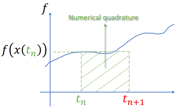
- Advection: “Move” the fluid field (no external forces, just the simple version), solve
- External Forces (usually gravity accelaration, optional): evaluate
- Projection: make velocity field
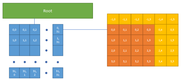
Grid
Spatial Discretization
Using Cell-centered Grids
(evenly distributed)
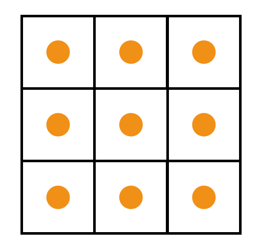
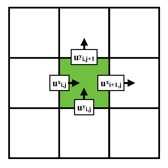
xxxxxxxxxxn, m = 3, 3u = ti.var(ti.f32, shape = (n, m)) # x-comp of velocityv = ti.var(ti.f32, shape = (n, m)) # y-comp of velocityp = ti.var(ti.f32, shape = (n, m)) # pressureUsing Staggered grids
Stored in various location (Red -
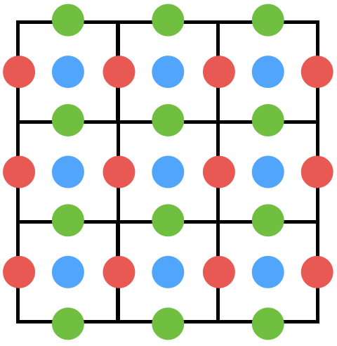 Red: 3x4; Green: 4x3; Blue: 3x3
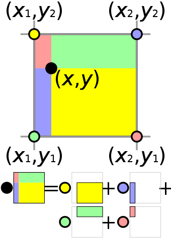
xxxxxxxxxxn, m = 3, 3u = ti.var(ti.f32, shape = (n+1, m)) # x-comp of velocityv = ti.var(ti.f32, shape = (n, m+1)) # y-comp of velocityp = ti.var(ti.f32, shape = (n, m)) # pressureBilinear Interpolation
Interpolate
Advection
Different Schemes: Trade-off between numerical viscosity, stability, performance and complexity
- Semi-Lagrangian Advection
- MacCormack / BFECC
- BiMocq2
- article Advection (PIC / FLIP / APIC / PolyPIC)
Semi-Lagrangian Advection
Scheme
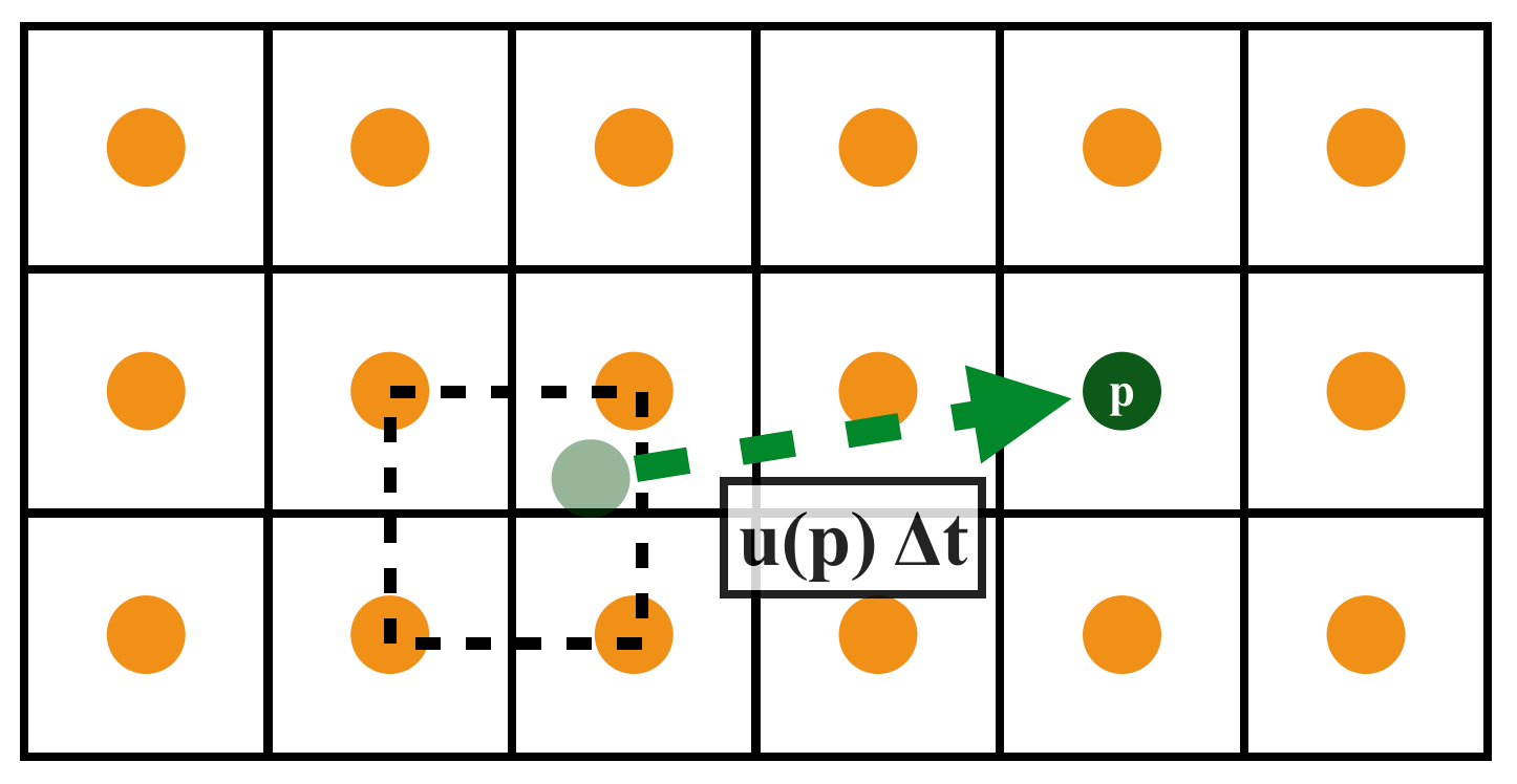
Velocity field constant, for very short time step
xxxxxxxxxx.funcdef semi_lagrangian(x, new_x, dt): for I in ti.grouped(x): # loop over all subscripts in x new_x[I] = sample_bilinear(x, backtrace(I, dt)) # backtrace means the prev. value of x at the prev. dt # (find the position of the prev. x value in this field, and do bilinear interpolation and give to new_x)Problem
velocity field not constant! -> Cause magnification / smaller / blur
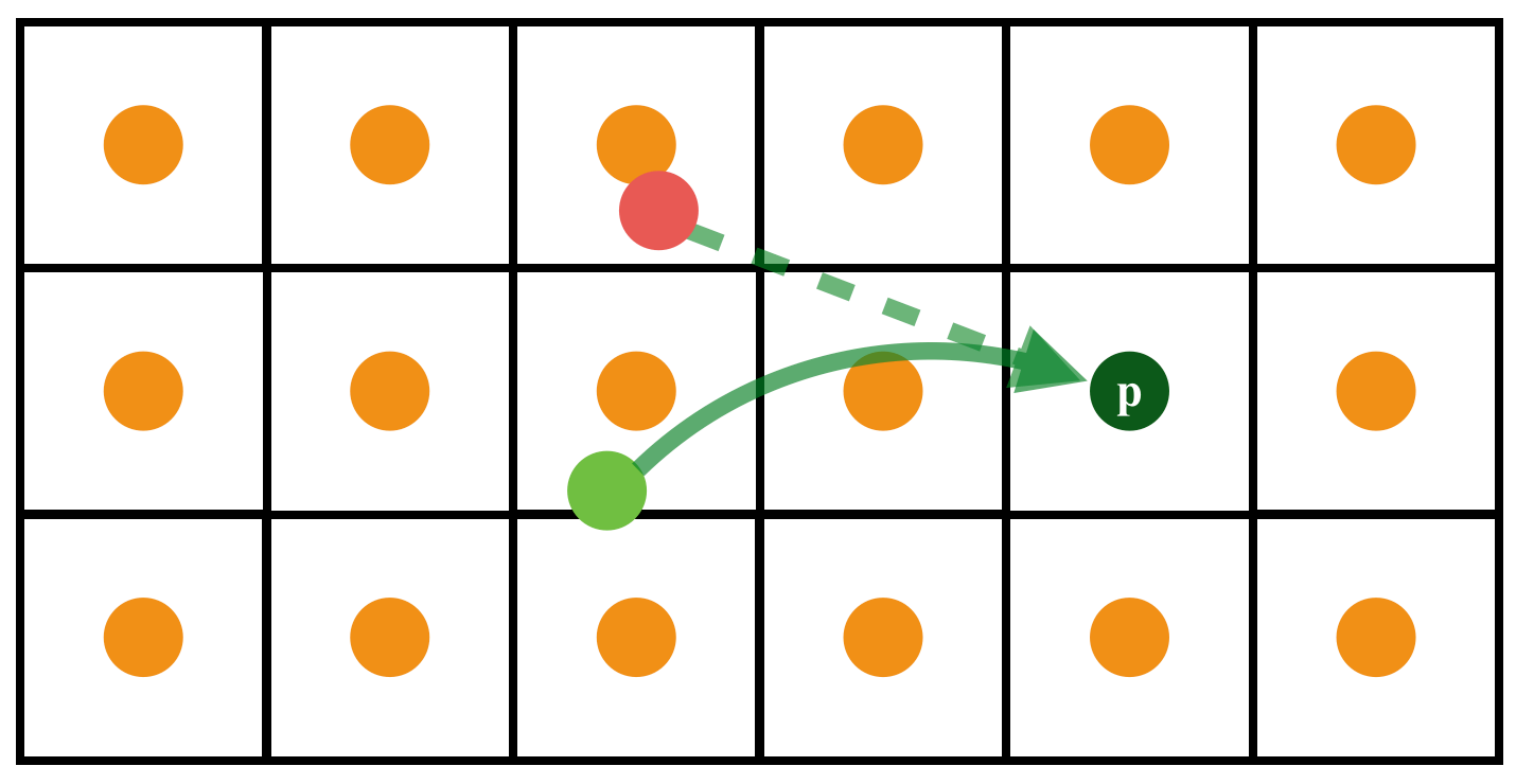
The real trajectory of material parcels can be complex (Red: a naive estimation of last position; Light gree: the true previous position.)
Solutions
(-> initial value problem for ODE, simply use the naive algorithm = forward Euler (RK1); to solve the problem can use RK2 scheme)
Forward Euler (RK1)
xxxxxxxxxxp -= dt * velocity(p)Explicit Midpoint (RK2)
xxxxxxxxxxp_mid = p - 0.5 * dt * velocity(p)p -= dt * velocity(p_mid)(Blur but no become smaller, usually enough for most computations)
RK3 (weighted average of 3 points)
xxxxxxxxxxv1 = velocity(p)p1 = p - 0.5 * dt * v1v2 = velocity(p1)p2 = p - 0.75 * dt * v2v3 = velocity(p2)p -= dt * (2/9 * v1 + 1/3 * v2 + 4/9 * v3)(Result similar to RK2)
~ Blur: Usually because of the use of bilinear interpolation (numerical viscosity / diffusion) (causes energy reduction) -> BFECC
BFECC / MacCormack
Scheme
BFECC: Back and Forth Error Compensation and Correction (Good reduction of blur especially for static region boundaries)
- Error Estimation:
- Apply the error (correction):
xxxxxxxxxx.funcdef maccormack(x, dt): # new_x = x*; new_x_aux = x**; semi_lagrangian(x, new_x, dt) # step 1 (forward dt) semi_lagrangian(new_x, new_x_aux, -dt) # step 2 (backward dt) for I in ti.grounped(x): new_x[I] = new_x[I] + 0.5 * (x[I] - new_x_aux[I]) # Error estimation (new_x = x^{final})Problem: Overshooting
~ Gibbs Phenomen at boundary because of this correction: 0.5 * (x[I] - new_x_aux[I])
Idea: Introduce a clipping function
xxxxxxxxxx....
for I in ti.grounped(x): new_x[I] = new_x[I] + 0.5 * (x[I] - new_x_aux[I]) # prev. codes if ti.static(mc_clipping): source_pos = backtrace(I, dt) min_val = sample_min(x, source_pos) max_val = sample_max(x, source_pos) if new_x[I] < min_val or new_x[I] > max_val: new_x[I] = sample_bilinear(x, source_pos) (Artifacts)
Chorin-Style Projection
To ensure the velocity field is divergence free after projection - Constant Volume (need linear solver - MGPCG)
Expand using finite difference in time (
Divergence (
): the total generation / sink of the fluid (+ for out, - for in). For actual (imcompressible) fluid flow: $\cur Curl (
): Clockwise - ; Counter clockwise -
Want: find a
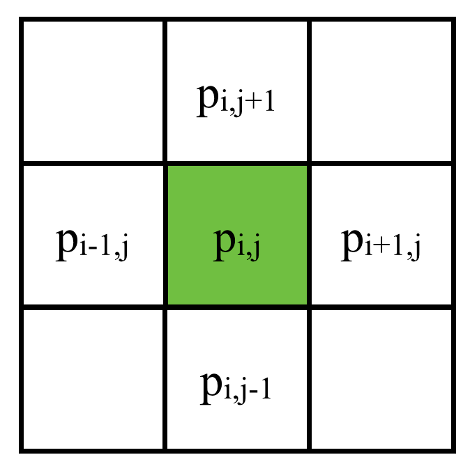
Poisson’s Equation
(
If
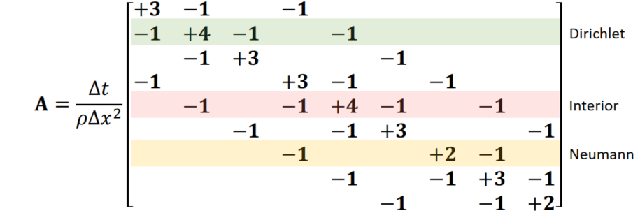
Spatial Discretization (2D)
Discretize on a 2D grid: (central differential, 5 points)
Linear System:
Divergency of velocity(速度的散度): Quantity of fluids flowing in / out: Flows in = Negative; Flows out = Positive
Remind: Staggered Grid: x-componenets of u - vertical boundaries; y-comp: horizontal boundaries
Boundary Conditions
Dirichlet and Neumann boundaries
- Open (regard as air):
- Regard as solid:
Solving Large-scale Linear Systems
Direct solvers (e.g. PARDISO) - small linear system
Iterative solvers:
- Gauss-Seidel
- (Damped) Jacobi
- (Preconditioned) Krylov-subspace solvers (e.g. conjugate gradients)
(Good numerical solver are usually composed of different solvers)
Matrix Storage
Store
- As a dense matrix: e.g.
float A[1024][1024](doesn’t scale, but works for small matrices) - As a sparse matrix: (various formats: CSR, COO, ..)
- Don’t store it at all (Matrix-free, often the ultimate solution) (Fetching values costs much, so in graphics usually not store)
Krylov-subspace Solvers
- Conjugate gradients (CG) (Commonly used)
- Conjugate residuals (CR)
- Generalized minimal residual method (GMRES)
- Biconjugate gradient stabilized (BiCGStab)
Conjugate gradients
Basic Algorithm: (energy minimization)
Eigenvalues and Condition Numbers
Convergence related to condition numbers
Remind:
if
即
Condition Number
A smaller condition number causes faster convergence
Warm Starting
Starting with an closer initial guess results in fewer interations needed
Using
Preconditioning
Find an approximate operator
Common Preconditioners:
- Jacobi (diagonal) preconditioner
- Poisson preconditioner
- (incomplete) Cholesky decomposition
- Multigrid:
- Fast multipole method (FMM)
Multigrid preconditioned conjugate gradients (MGPCG)
Residual reduction very fast in several iterations
A. McAdams, E. Sifakis, and J. Teran (2010). “A Parallel Multigrid Poisson Solver for Fluids Simulation on Large Grids.”. In: Symposium on Computer Animation, pp. 65–73.
Taichi demo: 2D/3D multigrd: ti example mgpcg_advanced
Lecture 5 Poisson’s Equation and Fast Method
Poisson’s Equation and its Fundamental Solution
Using the view of PDE
For example: Gravitational Problem (势场满足密度的泊松方程)
If N particles in M points computaiton -> Required
Fast Summation
快速多级展开
M2M Transform
2D (Using Complex number to represent in coordinate):
Consider a source and its potential:
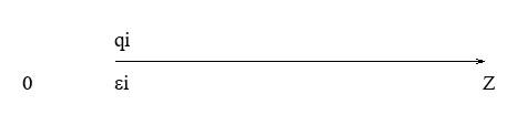
- Apply Taylor Expansion:
- Apply Taylor Expansion:
Multipole Expansion:
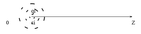 (every point in the cloud represeted as qj)
(来自 0 点的势作用之和 + 高阶项对于 Z 的影响(由形状))
将公式抽象(
One step further:
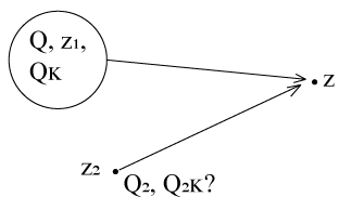
Problem: If we know M-Expansion at (electron cloud) Z1 (M1 = {z1, Q, Qk}), what is the M-Expansion at Z2 (M2 = {z2, Q2, Q2,k})?
Actually a M to M translation (from z1 to z2)
We want to obtain the coefficients from M1 , not qi’s
Recall
View Sources as Multipole:
Reveal “Multipole Expansion”
From “Multipoles” (every multipole - an electron) ~ M2M Transform
Compute bk with “Rest of terms”
xxxxxxxxxxstruct Multipole{ vec2 center; // central point (in coordinate) complex q[p]; // rest of terms (in complex)};//source charge is a special Multipole,//with center = charge pos, q0 = qi, q1…q4 =0
Multipole M2M(std::vector<Multipole> &qlist){ Multipole res; res.center = weightedAverageof(qlist[i].center*qlist[i].q[0]); // new center point (weighted average) q[0] = sumof(qlist[i].q[0]); // q0 terms for(k=1:p){ res.q[k]=0; for(j=0:qlist.size()) { res.q[k] += computeBk(qlist[i]); // compute bk function } } return res;}(Electrons - Multipoles and Multipole - Multipole)
For M2M Transform: Both z1 and z2 are far from Z; For M2L (Local pole ~ interpolation) Transform: z1 near Z
M2L Transform
If we know M-Expansion at c1 (M1 = {c1, Q, Qk}), what is the polynomial at z1, so that potentials at neighbor z can be evaluated.
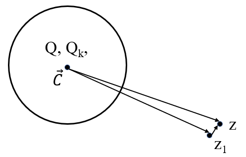
where H.O.T. is high order turbulence, from multipole to local pole
xxxxxxxxxxstruct Localpole{ vec2 center; complex b[p];};L2L Transform
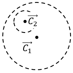
If we know L-Expansion at c1 (L1 = {c1, B}), what is the polynomial at c2, so that potentials at neighbor z around c2 can be evaluated? Honer Scheme
Comparison
- Multipole expansion: Coarsening
- Localpole expansion: Interpolation
26:00
—
Taichi Graphic Course S1 (NEW)
Lecture 0-2 is in the above notes
Lecture 3 Advanced Data Layout (21.10.12)
Advanced Dense Data Layouts
(ti.field() is dense and @ti.kernel is optimized for field => Data Oriented => focus on data-access / decouple the ds from computations)
CPU -> wall of computations; GPU / Parallel Frame -> wall of data access (memory access)
Packed Mode
Initiaized in
ti.init()default:
packed = False: do paddinga = ti.field(ti.i32, shape=(18,65)) # padded to (32, 128)packed = True: for simplicity (No padding)
Optimized for Data-access
1D fields:
Prefetched (every time access the memory -> slow): align the access order with the memory order
N-D fields: stored in our 1D memory: store as what it accesses
Ideal memory layout of oan N-D field (not matter line / col. / block major)
For example in C/C++:
xxxxxxxxxxint x[3][2]; // row-majorint y[2][3]; // col.-major (actually still 3x2)foo(){for (int i = 0; i < 3; i++) {for (int j = 0; j < 2; j++) {d_somthing(x[i][j]);}}for (int j = 0; j < 2; j++) {for (int i = 0; i < 3; i++) {do_somthing(y[j][i]);}}}
Upgrade ti.field()
From shape to ti.root
xxxxxxxxxxx = ti.Vector.field(3, ti.f32, shape = 16)change to:
xxxxxxxxxxx = ti.Vector.field(3, ti.f32)ti.root.dense(ti.i, 16).place(x)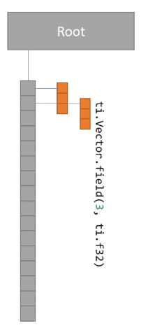
One step futher:
xxxxxxxxxxx = ti.field(ti.i32)ti.root.dense(ti.i, 4).dense(ti.j, 4).place(x)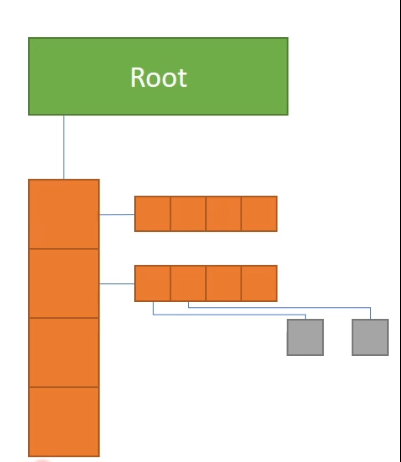
SNode: Structure node
An SNode Tree:
xxxxxxxxxxti.root # the root of the SNode-tree.dense() # a dense container decribing shape.place(ti.field()) # a field describing cell data...
A Taichi script uses dense equiv. to the above C/C++ codes
xxxxxxxxxxx = ti.field(ti.i32)y = ti.field(ti.i32)ti.root.dense(ti.i, 3).dense(ti.j, 2).place(x) # row-majorti.root.dense(ti.j, 2).dense(ti.i, 3).place(y) # col.-major
.kerneldef foo(): for i, j in x: do_something(x[i, j]) for i, j in y: do_something(y[i, j])Row & Column Majored Fields
Col: 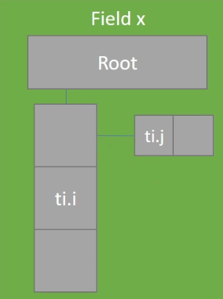 Row:
Row: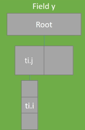
Access: struct for (the access order will altered for row and col. -majored)
Example: loop over ti.j first (row-majored)
xxxxxxxxxximport taichi as titi.init(arch = ti.cpu, cpu_max_num_threads=1)
x = ti.field(ti.i32)ti.root.dense(ti.i, 3).dense(ti.j, 2).place(x)# row-major
.kerneldef fill(): for i,j in x: x[i, j] = i*10 + j .kerneldef print_field(): for i,j in x: print("x[",i,",",j,"]=",x[i,j],sep='', end=' ') fill()print_field() Special Case (dense after dense)
Hierachical 1-D field (block storage)
- Access like a 1-D field
- Store like a 2-D field (in blocks)
xxxxxxxxxxx = ti.field(ti.i32)ti.root.dense(ti.i, 4).dense(ti.i, 4).place(x) # hierarchical 1-D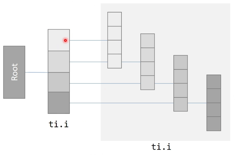
Block major
e.g. for 9-point stencil
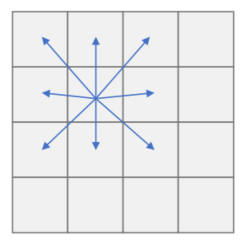
xxxxxxxxxxx = ti.field(ti.i32)ti.root.dense(ti.ij, (2,2)).dense(ti.ij, (2,2)).place(x) # Block major hierarchical layout, size = 4x4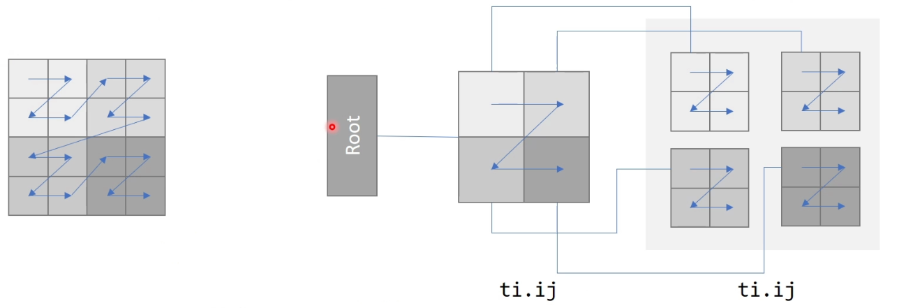
Compare to flat layouts:
xxxxxxxxxxz = ti.field(ti.i32, shape = (4,4))# row-majored flat layout; size = 4x4Array of Structure (AoS) and Structure of Arrays (SoA)
xxxxxxxxxxstruct S1 { int x[8]; int y[8]; } S1 soa;xxxxxxxxxxstruct S2 { int x; int y; } S2 aos[8];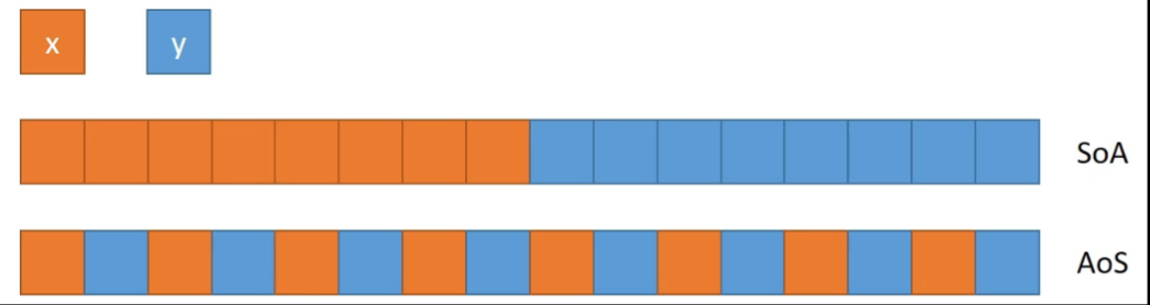
Switching: ti.root.dense(ti.i, 8).place(x,y) -> ti.root.dense(ti.i, 8).place(x) + ti.root.dense(ti.i, 8).place(y)
Sparse Data Layouts
SNode Tree (Extended)
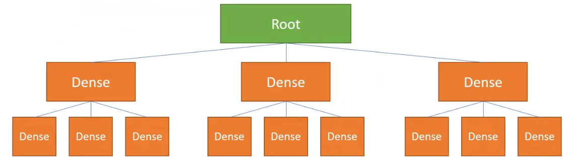
- root
- dense: fixed length contiguous array
- bitmasked: similar to dense, but it also uses a mask to maintain sparsity info
- pointer: stores pointers instead of the whole structure to save memory and maintain sparsity
Dense SNode-Tree:
Pointer
But the space occupation rate could be low -> use pointer (when no data in the space a pointer points -> set to 0)
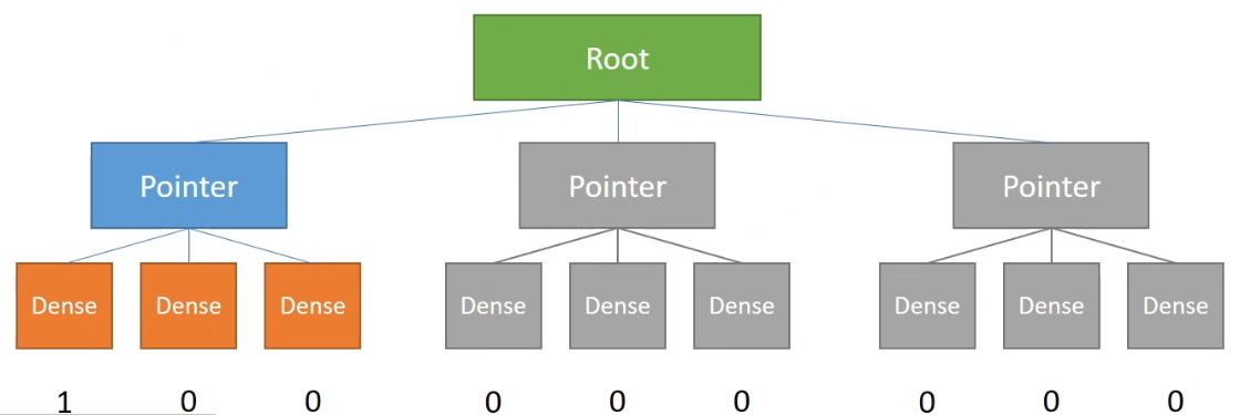
Activation
Once writing an inactive cell: x[0,0] = 1 (activate the whole block the pointer points to (cont. memory))
If print => inactivate will not access and return 0
Pointer in Pointer
Actually ok but can be a waste of memory (pointer = 64 bit / 8 bytes). can also break cont. in space
Bitmasked
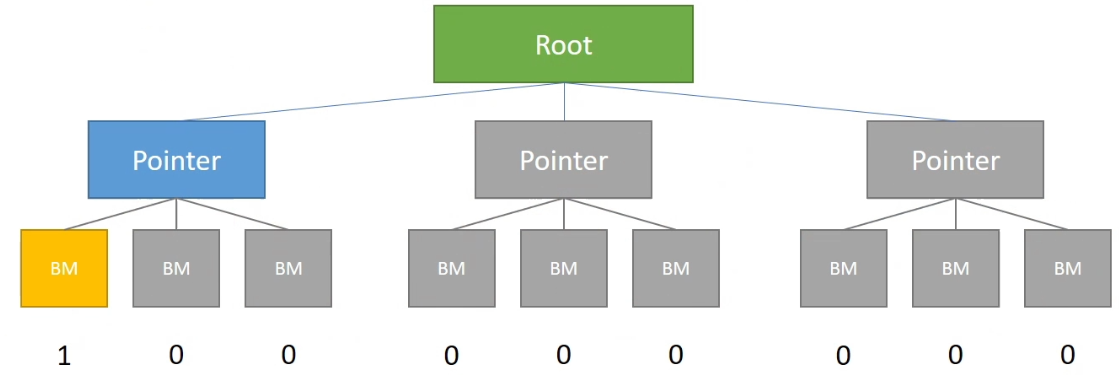
The access / call is similar to a dense block. Cost 1-bit-per-cell extra but can skip some …
API
Check activation status:
ti.is_active(snode, [i, j, ...])e.g.:
ti.is_active(block1, [0]) # = TrueActivate / Deactivate cells:
ti.activate/deactivate(snode, [i,j])Deactivate a cell and its children:
snode.deactivate_all()Compute the index of ancestor
ti.rescale_index(snode/field, ancestor_snode, index)e.g.:
ti.rescale_index(block2, block1, [4]) # = 1
Put Together
Example
A column-majored 2x4 2D sparse field:
xxxxxxxxxxx = ti.field(ti.i32)ti.root.pointer(ti.j,4).dense(ti.i,2).place(x)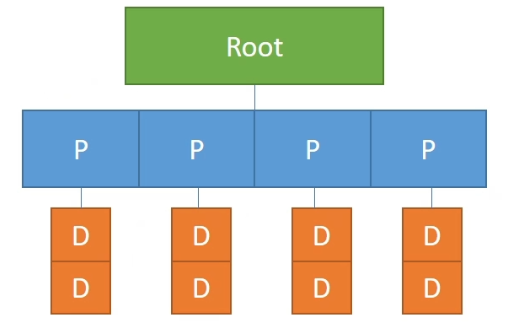
A block-majored (block size = 3) 9x1 1D sparse field:
xxxxxxxxxxx = ti.field(ti.i32)ti.root.pointer(ti.i,3).bitmasked(ti.i,3).place(x)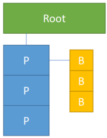
Lecture 4 Sparse Matrix, Debugging and Code Optimization (21.10.19)
Sparse Matrix and Sparse Linear Algebra
Naive Taichi Implementation: hard to maintain
Build a Sparse Matrix
Sparse Matrix Solver:
ti.SparseMatrixBuilder()(Use triplet arrays to store the line / col / val)xxxxxxxxxxn = 4K = ti.SparseMatrixBuilder(n, n, max_num_triplets=100).kerneldef fill(A: ti.sparse_matrix_builder()):for i in range(n):A[i, i] += 1Fill the builder with the matrices’ data:
xxxxxxxxxxfill(K)print(">>>> K.print_triplets()")K.print_triplets()# outputs:# >>>> K.print_triplets()# n=4, m=4, num_triplets=4 (max=100)(0, 0) val=1.0(1, 1) val=1.0(1, 2) val=1.0(3, 3) val=1.0Create sparse matrices from the builder
xxxxxxxxxxA = K.build()print(">>>> A = K.build()")print(A)# outputs:# >>>> A = K.build()# [1, 0, 0, 0]# [0, 1, 0, 0]# [0, 0, 1, 0]# [0, 0, 0, 1]
Sparse Matrix Operations
- Summation:
A + B - Subtraction:
A - B - Scalar Multiplication:
c * AorA * c - Element-wise Multiplication:
A * B - Matrix Multiplication:
A @ B - Matrix-vector multiplication:
A @ b - Transpose:
A.transpose() - Element Access:
A[i, j]
Sparse Linear Solver
xxxxxxxxxx# factorizesolver = ti.SparseSolver(solver_type="LLT") # def.: LL (Lower Tri.) Transpose (2); also could be "LDLT" / "LU"solver.analyze_pattern(A) # pre-factorizesolver.factorize(A) # factorization
# solvex = solver.solve(b) # (numpy) array
# check stats# if not, could be the factorization error (symmetric? ..)isSuccessful = solver.info()print(">>>> Solve sparse linear systems Ax = b with solution x")print(x)print(f">>>> Computation was successful?: {isSuccessful}")Example: Linear Solver(鸡兔同笼)
Given the amount of heads and legs to compute the amount of chicken and rabbit
If the problem is solved intuitively as a linear system
-> Use x = solver.solve(b)
Example: Linear Solver (Diffusion)
Finite Differential Method with FTCS Scheme
Spatially discretized:
Temporally discretized: (explicit)
xxxxxxxxxx.kerneldef diffuse(dt: ti.f32): c = dt * k / dx**2 for i,j in t_n: t_np1[i,j] = t_n[i,j] if i-1 >= 0: t_np1[i, j] += c * (t_n[i-1, j] - t_n[i, j]) if i+1 < n: t_np1[i, j] += c * (t_n[i+1, j] - t_n[i, j]) if j-1 >= 0: t_np1[i, j] += c * (t_n[i, j-1] - t_n[i, j]) if j+1 < n: t_np1[i, j] += c * (t_n[i, j+1] - t_n[i, j])Matrix Representation: (Explicit)
The temperature transfer function can be easier to express:
xxxxxxxxxxdef diffuse(dt: ti.f32): c = dt * k / dx**2 IpcD = I + c*D t_np1.from_numpy(IpcD@t_n.to_numpy()) # t_np1 = t_n + c*D*t_n .kerneldef fillDiffusionMatrixBuilder(A:ti.sparse_matrix_builder()): for i,j in ti.ndrange(n, n): count = 0 if i-1 >= 0: A[ind(i,j), ind(i-1,j)] += 1 count += 1 if i+1 < n: A[ind(i,j), ind(i+1,j)] += 1 count += 1 if j-1 >= 0: A[ind(i,j), ind(i,j-1)] += 1 count += 1 if j+1 < n: A[ind(i,j), ind(i,j+1)] += 1 count += 1 A[ind(i,j), ind(i,j)] += -countMatrix Representation: (Implicit)
xxxxxxxxxxdef diffuse(dt: ti.f32): c = dt * k / dx**2 ImcD = I - c*D # linear solve: factorize solver = ti.SparseSolver(solver_type="LLT") solver.analyze_pattern(ImcD) solver.factorize(ImcD) # linear solve: solve t_np1.from_numpy(solver.solve(t_n)) # t_np1 = t_n + c*D*t_np1 .kerneldef fillDiffusionMatrixBuilder(A:ti.sparse_matrix_builder()): for i,j in ti.ndrange(n, n): count = 0 if i-1 >= 0: A[ind(i,j), ind(i-1,j)] += 1 count += 1 if i+1 < n: A[ind(i,j), ind(i+1,j)] += 1 count += 1 if j-1 >= 0: A[ind(i,j), ind(i,j-1)] += 1 count += 1 if j+1 < n: A[ind(i,j), ind(i,j+1)] += 1 count += 1 A[ind(i,j), ind(i,j)] += -countNew Features (0.8.3+)
Sparse Matrix related features to ti.linalg
ti.SparseMatrixBuilder->ti.linalg.SparseMatrixBuilderti.SparseSolver->ti.linalg.SparseSolverti.sparse_matrix_builder()->ti.linalg.sparse_matrix_builder()
Debugging a Taichi Project
Print Results
Taichi still not supports break point debugging
Use run-time print in the taichi scope to check every part
The print order will not be in sequence unless
ti.syncis used to sync the program threadsPrint requires a system call. It can dramatically decrease the performance
Comma-separated parameters in the Taichi scope not supported
xxxxxxxxxx.kerneldef foo():print('a[0] = ', a[0]) # rightprint(f'a[0] = {a[0]}') # wrong, f-string is not supportedprint("a[0] = %f" % a[0]) # wrong, formatted string is not supported
Compile-time Print:
ti.static_printless performance loss (only at compile time)Print python-scope objects and constants in Taichi scope
xxxxxxxxxxx = ti.field(ti.f32, (2, 3))y = 1A = ti.Matrix([[1, 2], [3, 4], [5, 6]]).kerneldef inside_taichi_scope():ti.static_print(y)# => 1ti.static_print(x.shape)# => (2, 3)ti.static_print(A.n)# => 3for i in range(4):ti.static_print(A.m)# => 2# will only print once
Visualize Fields
Print a Taichi field / numpy array will truncate your results
xxxxxxxxxxx = ti.field(ti.f32, (256, 256))
.kerneldef foo(): for i,j in x: x[i,j] = (i+j)/512.0
foo() # print(x) # ok to print but not complete version (neglected mid elements)print(x.to_numpy().tolist()) # turn the field into a list and print the full versionThis method is hard to visualize -> use GUI / GGUI (normal dir / vel. dir / physics / …)
xxxxxxxxxxfoo()
gui = ti.GUI("Debug", (256, 256))while gui.running: gui.set_image(x) gui.show()Debug Mode
The debug mode is off by default
xxxxxxxxxxti.init(arch=ti.cpu, debug=True)for example: if
x = ti.field(ti.f32, shape = 4)and the field has not been def. and useprint(x[4])- Normal result:
x[4] = 0.0 - Debug mode:
RuntimeError(actually not defined yet. Not safe to use)
- Normal result:
Run-time Assertion
When debug mode is on, an assertion failure triggers a RuntimeError
xxxxxxxxxx.kerneldef do_sqrt_all():for i in x:assert x[i] >= 0 # test if larger than 0, if not show RuntimeErrorx[i] = ti.sqrt(x[i])But the assertion will be ignored in release mode. Real computing should not be in the assertion.
- Traceback:
line xx, in <module> func0()=> cannot trace to with function but only to the kernel (not good)
- Traceback:
Compile-time Assertion:
ti.static_assert(cond, msg=None)- No run-time costs;
- Useful on data types / dimensionality / shapes;
- Works on release mode
xxxxxxxxxx.funcdef copy(dst: ti.template(), src: ti.template()):ti.static_assert(dst.shape == src.shape, "copy() needs src and dst fields to be same shape")for I in ti.grouped(src):dst[I] = src[I]return x % 2 == 1Traceback: can trace which function is actually error
=>
excepthook=True(at initilization): Pretty mode (stack traceback)
Turn of Optimizations from Taichi
Turn off parallelization:
xxxxxxxxxxti.init(arch=ti.cpu, cpu_max_num_threads=1)Turn off advanced optimization
xxxxxxxxxxti.init(advanced_optimization=False)
Keep the Code Executable
Check the code everytime when finish a building block. Keep the entire codebase executable.
Other Problems
Data Race
- The for loop of the outermost scope is parallelized automatically, use
x += ()other than normalx = x + ()to apply atomic protection - In some neighbor update scenarioes, use another field other than just one field:
y[i] += x[i-1]because don’t know whether the neighbor had been updated or not
- The for loop of the outermost scope is parallelized automatically, use
Calling Python functions from Taichi scope
This triggers an undefined behaviour
Including functions from other imported python packages (numpy, for example) also cause this problem
xxxxxxxxxxdef foo():.......kerneldef bar():foo() # not from the Taichi scope => problemCopying 2 var in the Python Scope
b = a: for fields this behaviour could result in pointer points toaother than real copy (if change b, a will also be changed)=>
b.copy_from(a)The Data Types in Taichi should be Static
for example, in a loop, def.
sum = 0at first makes thesuman integer => precision lossThe Data in Taichi Have a Static Lexical Scope
xxxxxxxxxx.kerneldef foo():i = 20 # this is not useful even in Python scope (not recommended)for i in range(10): # Error...print (i)foo()Multiple Returns in a Single
@ti.funcnot Supportedxxxxxxxxxx.funcdef abs(x):if x >= 0: # res = xreturn x # if x < 0: res = -x (Correct) => return reselse:return -x # NOT SUPPORTEDData Access Using Slices not Supported
xxxxxxxxxxM = ti.Matrix(4, 4)...M_sub = M[1:2, 1:2] # NOT SUPPORTEDM_sub = M[(1,2), (1,2)] # NOT SUPPORTED
Optimizing Taichi Code
Performance Profiling
-> Amdahl’s Law (for higher run-time cost optimization will be more valueable)
Profiler
- Enable Taichi’s kernel profiler:
ti.init(kernel_profiler=True, arch=ti.gpu) - Output the profiling info:
ti.print_kernel_profile_info('count')(At last) - Clear profiling info:
ti.clear_kernel_profile_info()(Useful for neglecting the runtime costs before the real-wanted loop)
Demo
xxxxxxxxxx=========================================================================Kernel Profiler(count) @ CUDA=========================================================================[ % total count | min avg max ] Kernel name-------------------------------------------------------------------------[ 82.20% 0.002 s 17x | 0.090 0.105 0.113 ms] computeForce_c38_0_kernel_8_range_for [<- COSTS MOST][ 3.90% 0.000 s 17x | 0.002 0.005 0.013 ms] matrix_to_ext_arr_c14_1_kernel_12_range_for[ 3.17% 0.000 s 17x | 0.003 0.004 0.004 ms] computeForce_c34_0_kernel_5_range_for[ 2.17% 0.000 s 17x | 0.002 0.003 0.004 ms] matrix_to_ext_arr_c14_0_kernel_11_range_for[ 2.16% 0.000 s 17x | 0.002 0.003 0.004 ms] update_c36_0_kernel_9_range_for[ 2.09% 0.000 s 17x | 0.002 0.003 0.004 ms] computeForce_c34_0_kernel_6_range_for[ 2.05% 0.000 s 17x | 0.002 0.003 0.003 ms] update_c36_1_kernel_10_range_for[ 1.98% 0.000 s 17x | 0.002 0.003 0.003 ms] computeForce_c38_0_kernel_7_range_for[ 0.28% 0.000 s 2x | 0.002 0.003 0.004 ms] jit_evaluator_2_kernel_4_serial-------------------------------------------------------------------------[100.00%] Total execution time: 0.002 s number of results: 9=========================================================================
Performance Tuning Tips
BG: Thread hierarchy of Taichi in GPU
- Iteration (Orange): each iteration in a for-loop
- Thread (Blue): the minimal parallelizable unit
- Block (Green): threads are grouped in blocks with shared block local storage (Yellow)
- Grid (Grey): the minimal unit that being launched from the host
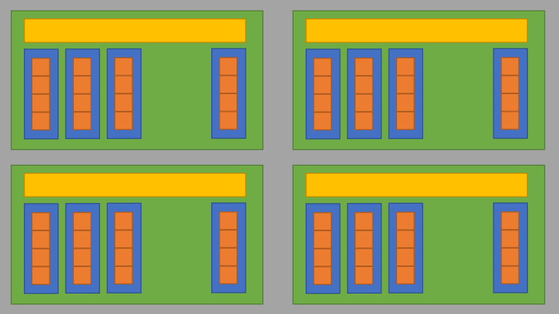
The Block Local Storage (BLS)
- Implemented using the shared memory in GPU
- Fast to read/write but small in size
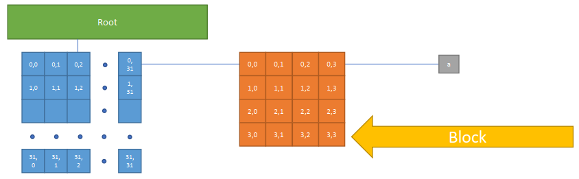
Block Size of an hierarchically defined field (SNode-tree):
xxxxxxxxxxa = ti.field(ti.f32)# 'a' has a block size of 4x4ti.root.pointer(ti.ij, 32).dense(ti.ij, 4).place(a)bls_size = 4 x 4 (x 4 Bytes) = 64 Bytes (Fast)
Decide the size of the blocks
ti.block_dim() before a parallel for-looop
(default_block_dim = 256 Bytes)
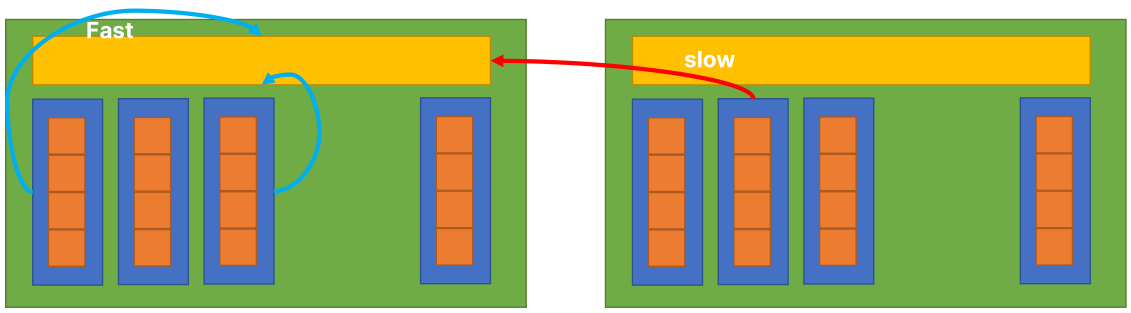
xxxxxxxxxx.kerneldef func(): for i in range(8192): # no decorator, use default settings ... ti.block_dim(128) # change the property of next for-loop: for i in range(8192): # will be parallelized with block_dim=256 ... for i in range(8192): # no decorator, use default settings ...Cache Most Freq-Used Data in BLS Manually
ti.block_local()
when a data is very important (actually in our case some neighbor will be counted as well)
xxxxxxxxxxa = ti.field(ti.f32)# `a` has a block size of 4x4ti.root.pointer(ti.ij, 32).dense(ti.ij, 4).place(a)
.kerneldef foo(): # Taichi will cache `a` into the CUDA shared memory ti.block_local(a) for i, j in a: print(a[i - 1, j], a[i, j + 2])bls_size = 5 x 6 (x 4 Bytes) = 120 Bytes (the overlapped part will be cached in different bls)
Lecture 5 Procedural Animation (21.10.26)
Procedure Animation in Taichi
Steps
- Setup the canvas
- Put colors on the canvas
- Draw a basic unit
- Repeat the basic units (tiles / fractals)
- Animate the pictures
- Introduce some randomness (chaos)
Demo: Basic Canvas Creation
xxxxxxxxxximport taichi as titi.init(arch = ti.cuda)
res_x = 512res_y = 512pixels = ti.Vector.field(3, ti.f32, shape=(res_x, res_y))
.kerneldef render(): # draw sth on the canvas for i, j in pixels: color = ti.Vector([0.0, 0.0, 0.0]) # init the canvas to black pixels[i, j] = color gui = ti.GUI("Canvas", res=(res_x, res_y))
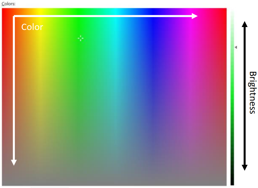
for i in range(100000): render() gui.set_image(pixels) gui.show()Colors
Add color via a for-loop
xxxxxxxxxx.kerneldef render(t:ti.f32): for i,j in pixels: r = 0.5 * ti.sin(float(i) / res_x) + 0.5 g = 0.5 * ti.sin(float(i) / res_y + 2) + 0.5 b = 0.5 * ti.sin(float(i) / res_x + 4) + 0.5 color = ti.Vector([r, g, b]) pixels[i, j] = colorBasic Unit
Draw a circle
xxxxxxxxxx.kerneldef render(t:ti.f32): for i,j in pixels: color = ti.Vector([0.0, 0.0, 0.0]) # init to black pos = ti.Vector([i, j]) center = ti.Vector([res_x/2.0, res_y/2.0]) r1 = 100.0 r = (pos - center).norm() if r < r1: color = ti.Vector([1.0, 1.0, 1.0]) pixels[i, j] = colorHelper Functions
Step
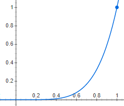
xxxxxxxxxx.funcdef step(edge, v):ret = 0.0if (v < edge): ret = 0.0else: ret = 1.0return retLinearstep (ramp)
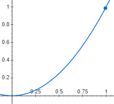
xxxxxxxxxx.funcdef linearstep(edge1, edge2, v):assert(edge1 != edge2)t = (v - edge1) / float(edge2 - edge1)t = clamp(t, 0.0, 1.0)return t # can also do other interpolation methods# such as: return (3-2*t) * t**2 (plot below)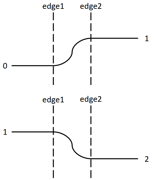
Demo: Basic Unit with Blur
xxxxxxxxxx.funcdef circle(pos, center, radius, blur): r = (pos - center).norm() t = 0.0 if blur > 1.0: blur = 1.0 if blur <= 0.0: t = 1.0-hsf.step(1.0, r/radius) else: t = hsf.smoothstep(1.0, 1.0-blur, r/radius) return t
.kerneldef render(t:ti.f32): for i,j in pixels: ... c = circle(pos, center, r1, 0.1) color = ti.Vector([1.0, 1.0, 1.0]) * c pixels[i, j] = color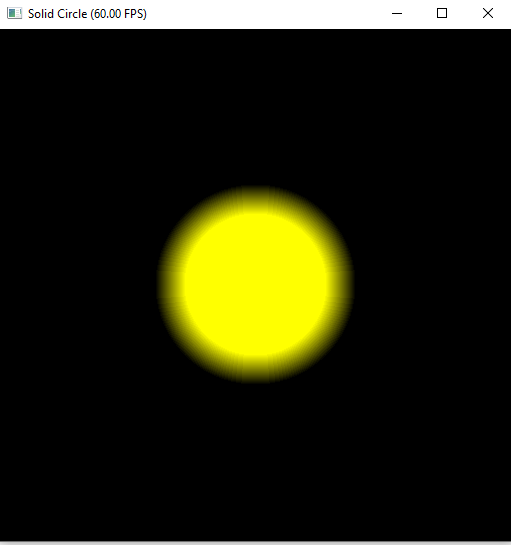
Repeat the Basic Units: Tiles
xxxxxxxxxx.kerneldef render(t:ti.f32): # draw something on your canvas for i,j in pixels: color = ti.Vector([0.0, 0.0, 0.0]) # init your canvas to black tile_size = 64 center = ti.Vector([tile_size//2, tile_size//2]) radius = tile_size//2 pos = ti.Vector([hsf.mod(i, tile_size), hsf.mod(j, tile_size)]) # scale i, j to [0, tile_size-1] c = circle(pos, center, radius, 0.1) color += ti.Vector([1.0, 1.0, 1.0])*c pixels[i,j] = color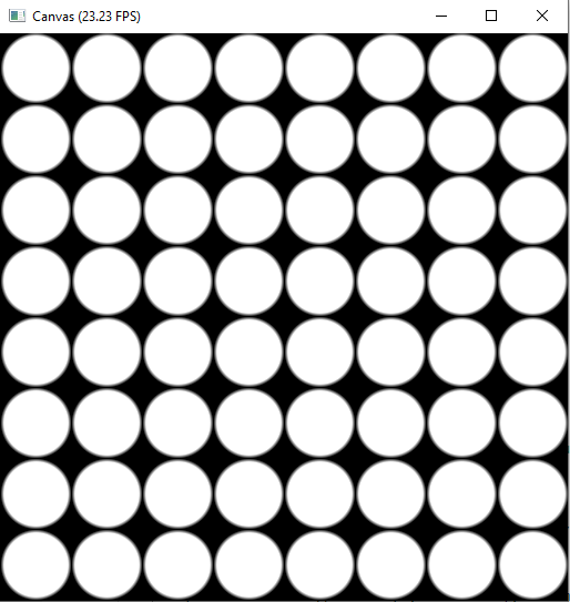
Repeat the Basic Units: Fractals
xxxxxxxxxx.kerneldef render(t:ti.f32): # draw something on your canvas for i,j in pixels: color = ti.Vector([0.0, 0.0, 0.0]) # init your canvas to black tile_size = 16 for k in range(3): center = ti.Vector([tile_size//2, tile_size//2]) radius = tile_size//2 pos = ti.Vector([hsf.mod(i, tile_size), hsf.mod(j, tile_size)]) # scale i, j to [0, tile_size-1] c = circle(pos, center, radius, 0.1) color += ti.Vector([1.0, 1.0, 1.0])*c color /= 2 tile_size *= 2 pixels[i,j] = color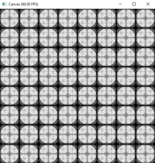
Animate the Picture
xxxxxxxxxx.kerneldef render(t:ti.f32): # this t represents time (or other par) and added in the followed expressions # draw something on your canvas for i,j in pixels: r = 0.5 * ti.sin(t+float(i) / res_x) + 0.5 g = 0.5 * ti.sin(t+float(j) / res_y + 2) + 0.5 b = 0.5 * ti.sin(t+float(i) / res_x + 4) + 0.5 color = ti.Vector([r, g, b]) pixels[i, j] = color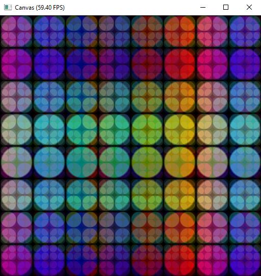
Introduce randomness (chaos)
y = rand(x)/y = ti.random()(white noise, need to find a balance in smooth and chaos)make in [0, 1]:
y = fract(sin(x) * 1.0)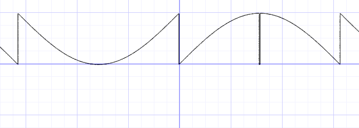
scale up:
y = fract(sin(x) * 10000.0)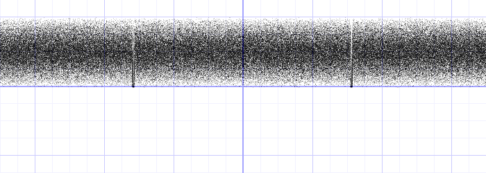
xxxxxxxxxxblur = hsf.fract(ti.sin(float(0.1 * t + i // tile_size * 5 + j // tile_size * 3)))c = circle (pos, center, radius, blur)
The Balance: Perlin noise (huge randomness but continuous in smaller scales)
-> shadertoy.com
Lecture 6 Ray Tracing (21.11.2)
Basis of Ray Tracing
Rendering Types
- Realtime Rendering: Rasterization
- Offline Rendering: Ray Tracing
Assumptions of Light Rays
Light rays
- go in straight lines
- do not collide with each other
- are reversible
Applying Ray Tracing (Color)
In color finding, option 1-2 usually use rasterization than RT. The classical RT is option 3 and the modern RT is actually option 4 (path tracing)
Option 1: The Color of the Object
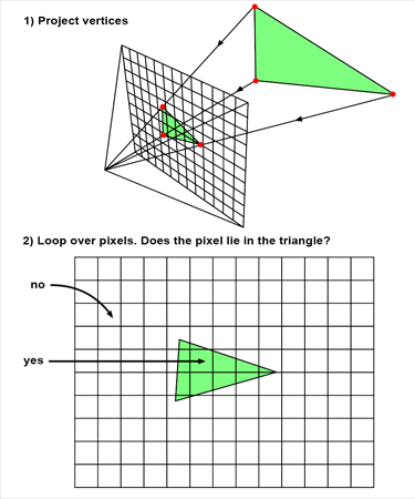
For 256x128:
Ray-tracing style:
- Generate 256x128 rays in 3D
- Check Ray-triangle intersection 256x128 times in 3D
Rasterization style
- Project 3 points into the 2D plane
- Check if a point is inside the triangle 256x128 times in 2D
Flat-looking Results
Cannot tell the materials using their colors
What we see = color * brightness
Option 2: Color + Shading
Lambertian Reflectance Model
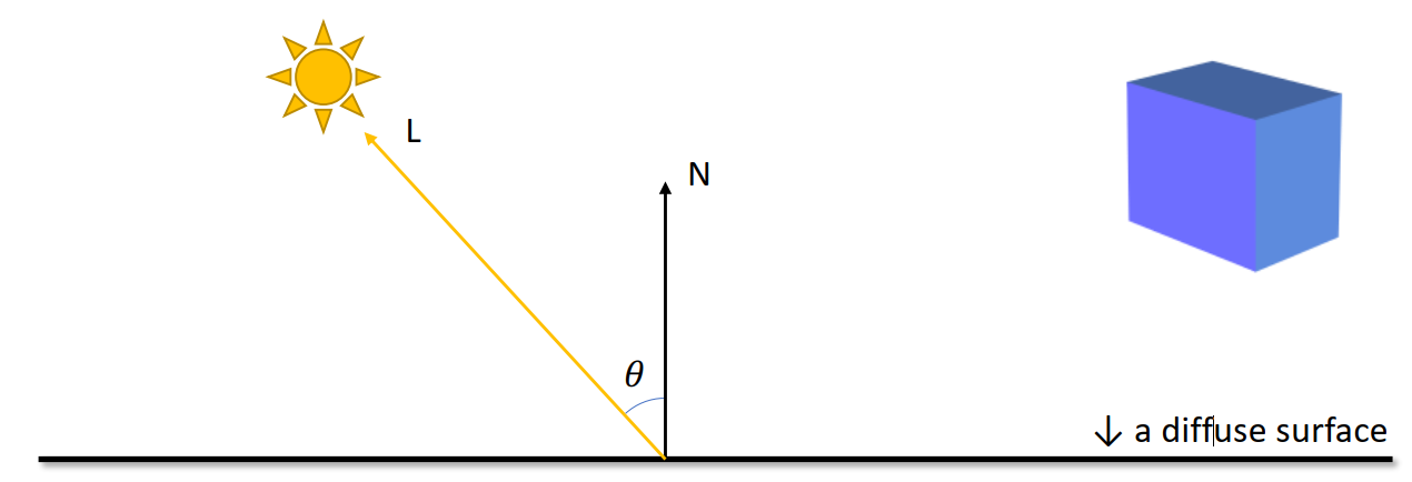
Brightness =
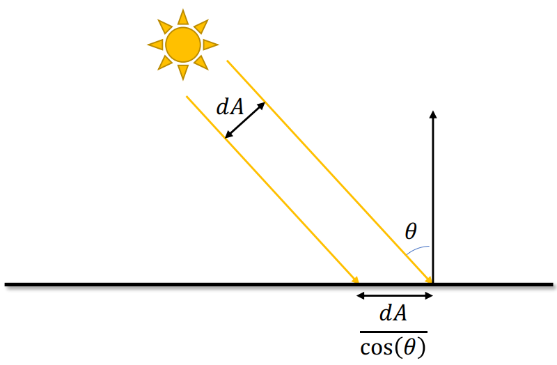
The larger
Results with Lambertian
Looks like 3D, but still lack of the specular surfaces
Phong Reflectance Model
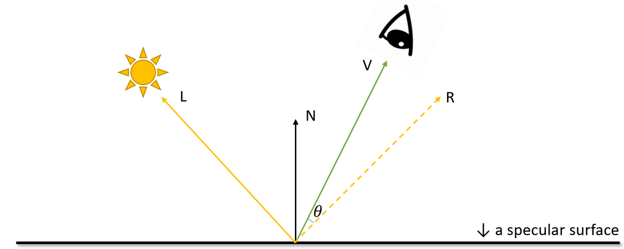
Brightness =
For higher
Blinn-Phong Reflectance Model
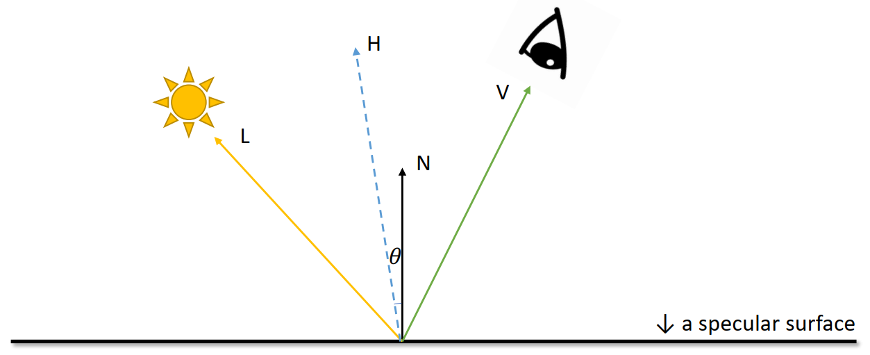
Brightness =
Blinn-Phong Shading Model
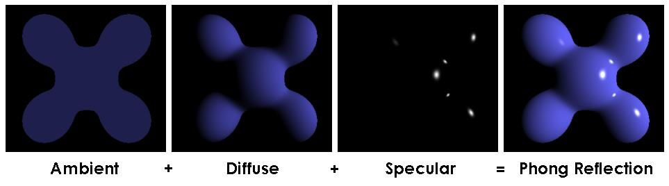
Results with Blinn-Phong
Shining but floating, no glassy like
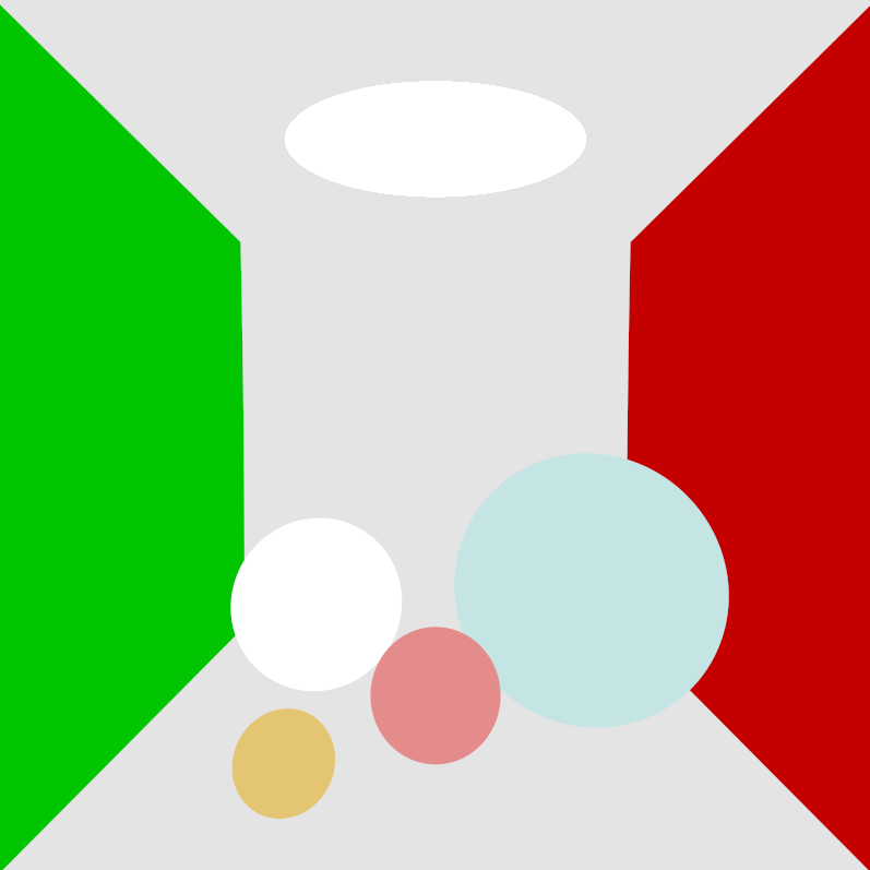
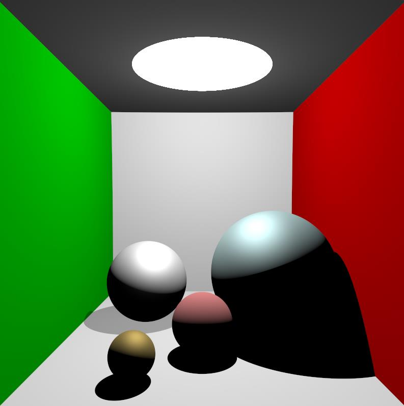
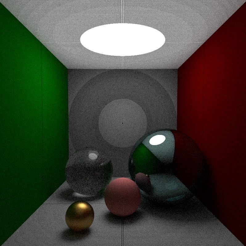
Option 3: The Whitted-Style Ray Tracer
-> Shadow / Mirror / Dielectric
The Whitted-Style
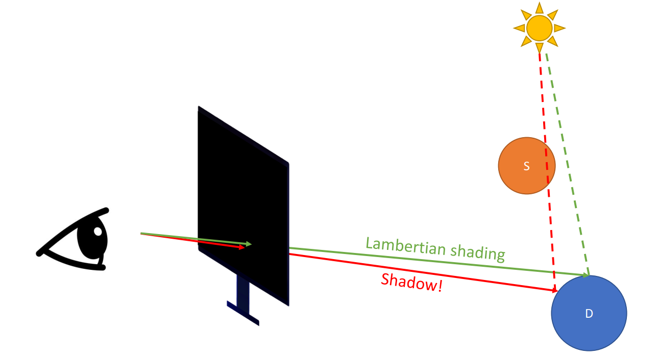
Since we have partially tranparent objects (the one with a gray shadow)
Refraction + Reflection (Recursive)
-> not easy to program
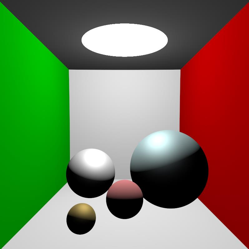
Problems
- Ceiling not lightened by the big light
- The huge light source only creates hard shadows (should be softer)
- No specular spots of the light on the ground through the transparent objects
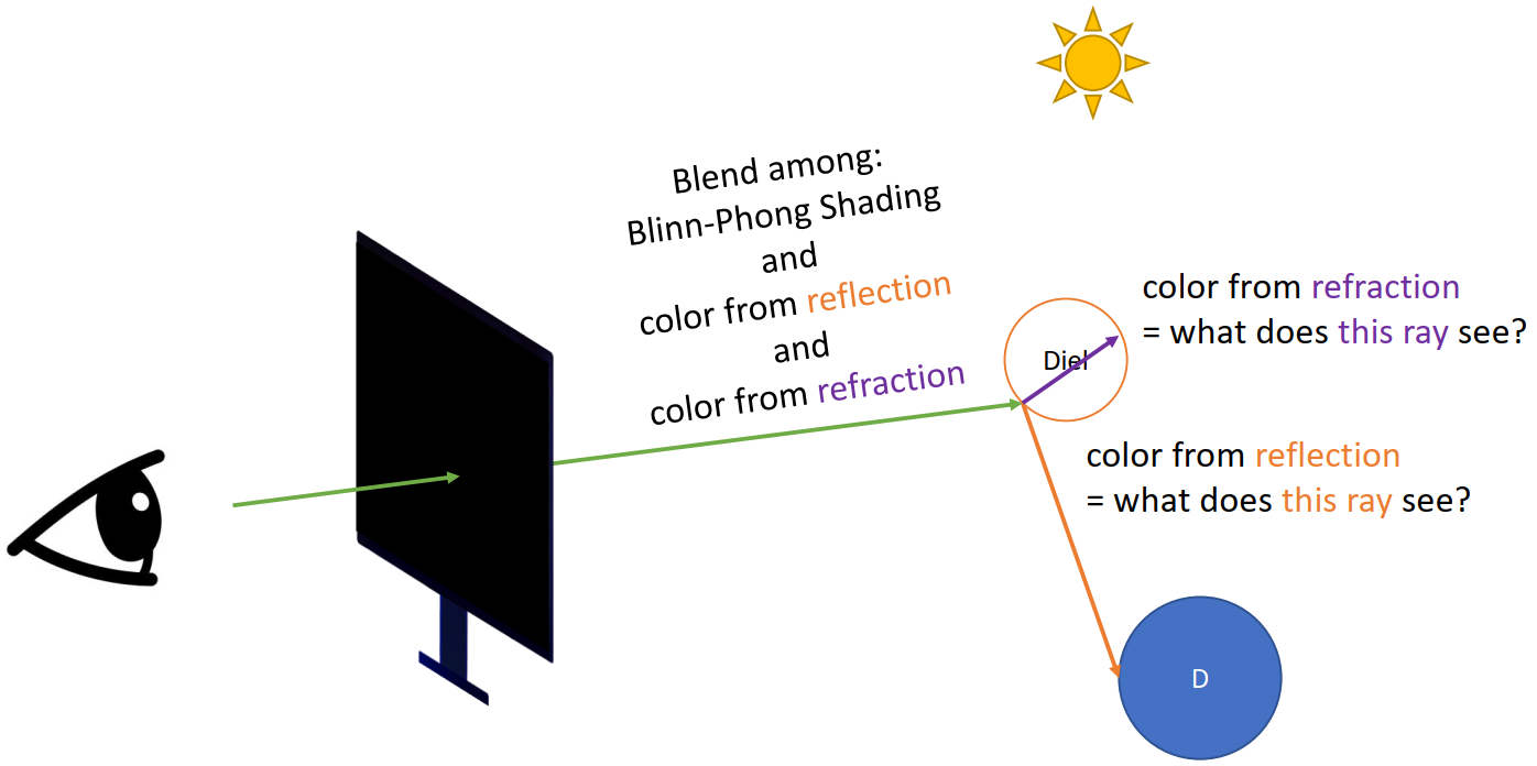
Option 4: Path Tracer (Modern)
From Previous Approaches
Shading Models:
- The brightness matters
The Whitted-Style Ray Tracing:
- Getting color recursively: what color does this ray see?
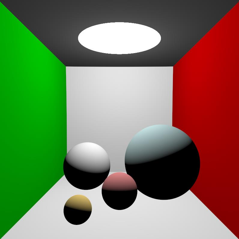
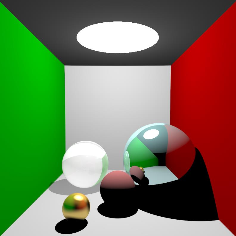
Global Illumination (GI)
With GI, diffuse surface will still scatter rays as well. Without GI, if not shined from the light source directly, it has fully dark shadow
An “unified” model for different surfaces:
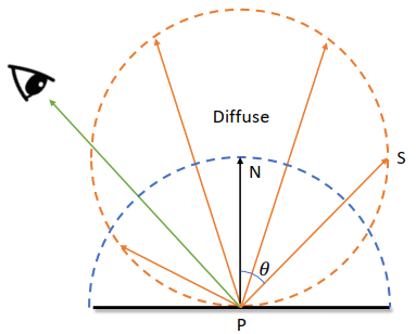
| Diffuse (Monte Carlo Method) | Specular | Dielectric |
|---|---|---|
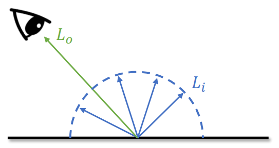 | 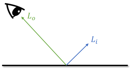 | 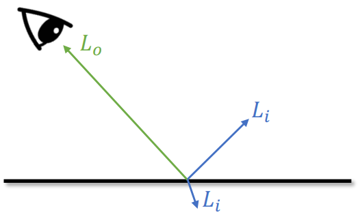 |
Monte Carlo Methdo: rely on repeated random sampling to obtain numerical results
All the collected weighted average color show the final color of a point
Problem in Sampling
Expensive (if
Noisy (if
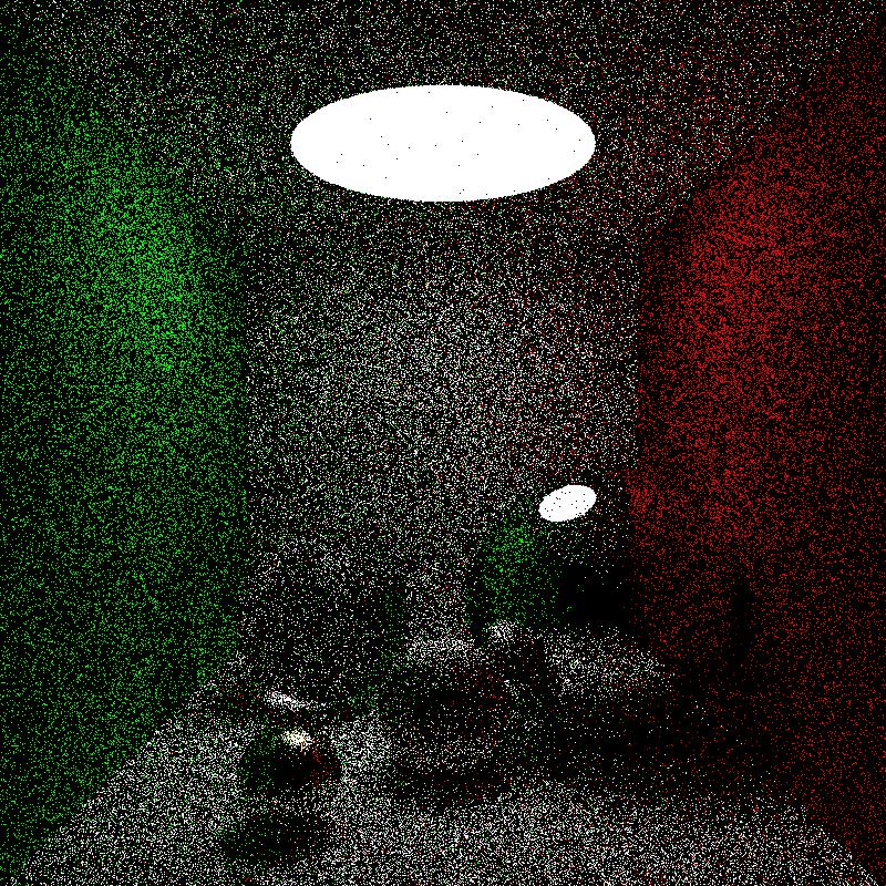
Solution:
Problems in Stop Criterion
The current stop criterion
Hit a light source
- Returns the color of the light source (usually [1.0, 1.0, 1.0])
Hit the bg (casted to the void)
- Returns the bg color (usually [0.0, 0.0, 0.0])
-> Problem: Infinity loops
Solution 1: Set depth of recursion (stop at the nth recursion): affects the illumination
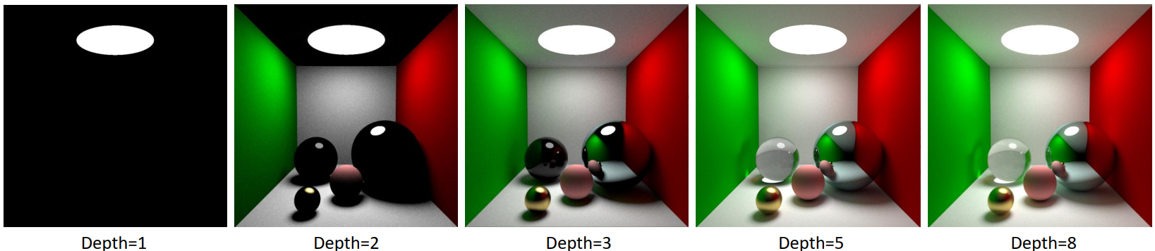
Solution 2: Russian Roulette
When asked “what color does the ray see”
Set a probability p_RR (for instance 90%)
Roll a dice (0-1)
if roll() > p_RR:
- stop recursion
- return 0
else:
- go on recursion: what is
- return
- go on recursion: what is
xxxxxxxxxxdef what_color_does_this_ray_see(ray_o, ray_dir): # original point and dirif (random() > p_RR):return 0else:flag, P, N, material = first_hit(ray_o, ray_dir, scene)if flag == False: # hit voidreturn 0if material.type == LIGHT_SOURCE: # hit light sourcereturn 1else: # recursiveray2_o = Pray2_dir = scatter(ray_dir, P, N)# the cos(theta) in DIFFUSE is hidden in the scatter functionL_i = what_color_does_this_ray_see(ray2_o, ray2_dir)L_o = material.color * L_i / p_RRreturn L_o
Core Ideas Summary
- Diffuse surfaces scatter light rays as well: Monte Carlo
- Every hit results in ONE scattered ray: But we sample every pixel multiple times
- Add the stop criterion: Russian Roulette (Depth caps are usually enabled too)
Further Readings
Radiometry
The rendering equation
Lecture 7 Ray Tracing 2 (21.11.9)
Recap
Color
- RGB Channels
- Range
- As a “filter”
Brightness:
- Power per unit solid angle per unit projected area
- Range
- Called Radiance in Radiometry
- Power per unit solid angle per unit projected area
What we see = Color * Brightness
What we see after multiple bounces = Color * Color * … * Brightness (Ray tracing)
Ray-casting from Camera/Eye
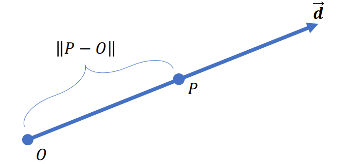
Ray
Ray is a line def by its origin (
Camera/Eye and Monitor
Positioning camera / eye
xxxxxxxxxxlookfrom[None] = [x, y, z]Orienting camera / eye
xxxxxxxxxxlookat[None] = [x, y, z]Placing the screen
xxxxxxxxxx# center pass through lookat-lookfrom# Perpendicular with lookat-lookfrom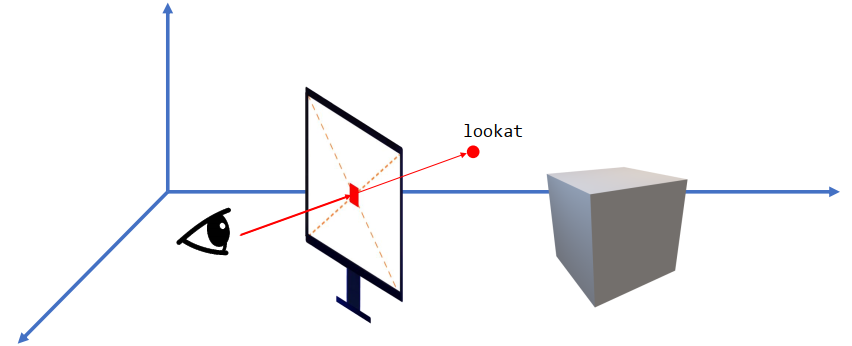
xxxxxxxxxxdistance = 1.0Orienting the screen (up vector)
xxxxxxxxxxup[None] = [0.0, 1.0, 0.0]Size of the screen (Field of View)
The FOV setting to match to the corresponding FOV of the real life will be better (i.e. smaller monitor / farther from the screen -> smaller FOV)
xxxxxxxxxxtheta = 1.0/3.0 * PIhalf_height = ti.tan(theta / 2.0) * distancehalf_width = aspect_ratio * half_height * distance # can also use another FOV to control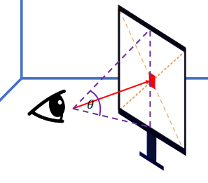
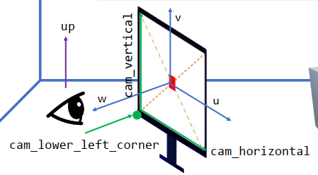
xxxxxxxxxxw = (lookfrom[None]-lookat[None]).normalized()u = (up[None].cross(w)).normalized()v = w.cross(u)xxxxxxxxxxcam_lower_left_corner[None] = (lookfrom[None] - half_width * u - half_height * v – w)* distancecam_horizontal[None] = 2 * half_width * u * distancecam_vertical[None] = 2 * half_height * v * distance
Ray-casting
xxxxxxxxxxu = float(i)/res_xv = float(j)/res_y # uv in [0, 1]ray.direction = cam_lower_left_corner[None] + u * cam_horizontal[None] + v * cam_vertical[None] - lookfrom[None] 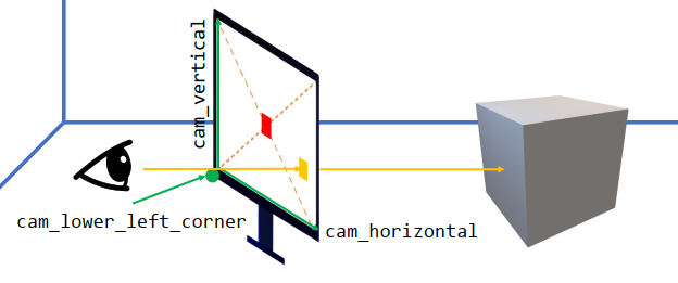
A pixel has its size as well -> + 0.5 pixels
xxxxxxxxxxu = float(i+0.5)/res_xv = float(j+0.5)/res_y # uv in (0, 1)Ray-object Intersection
Sphere
Sphere Intersection
Def of the sphere:
Intersection? :
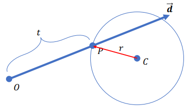
=>
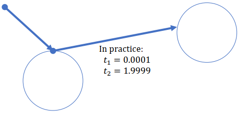
Find the smallest positive root
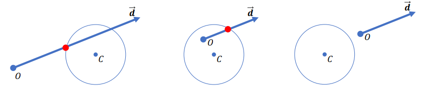
Problem: Shadow Acne (Caused by precision)
-> Want a slightly more positive number than 0:
For example in the following picture:
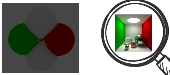
Cornell Box
Actually formed by 4 huge spheres other than using planes (more convenient)
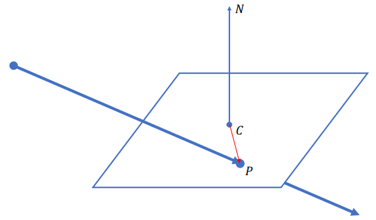
Plane
Ray-plane Intersection
Definition of a plane:
Intersection:
Ray-object Intersection
Implicit surfaces:
- Find its surface definition
- Plug the ray equation into the surface definition
- Look for the smallest positive
Polygonal surfaces: (Polygon meshes are usually made of triangles)
- Loop over all its polygons (usually triangles)
- Find the ray-polygon (triangle) intersection with the smallest positive
Sampling
Want to sample the directions of rays uniformly
Coordinates
Cartesian coordinates:
Polar coordinates:
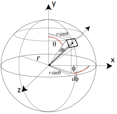
Sampling the Hemisphere Uniformly
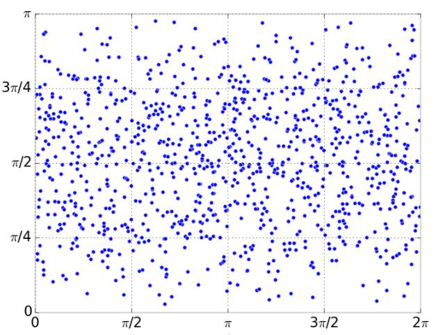
Attempt one:
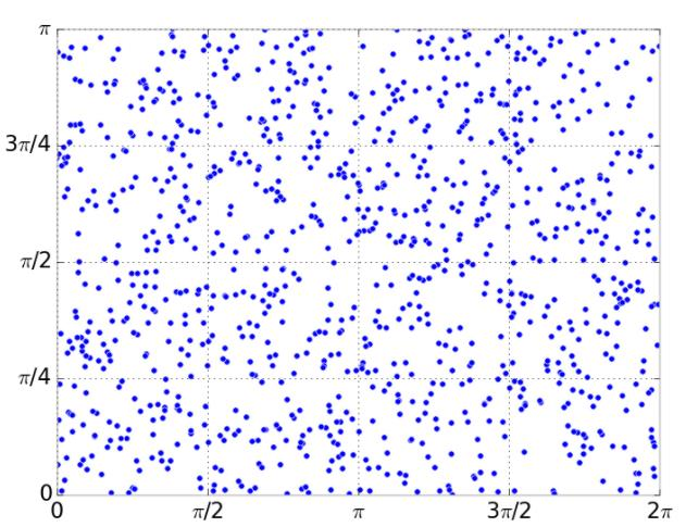
-> Uniform?: The probability of sampling is proportional to the surface area (differential surface element:
-> probability density function (p.d.f.)
The corrected attempt:
Negate the direction if against the normal
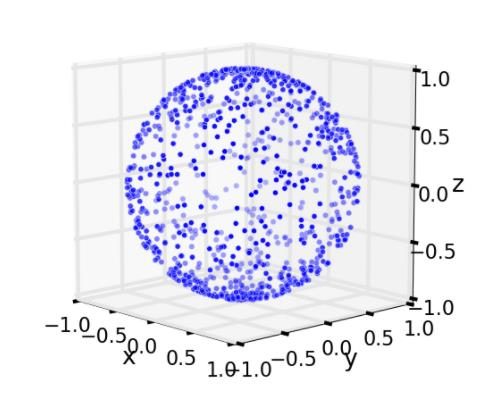
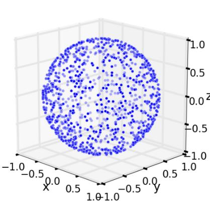
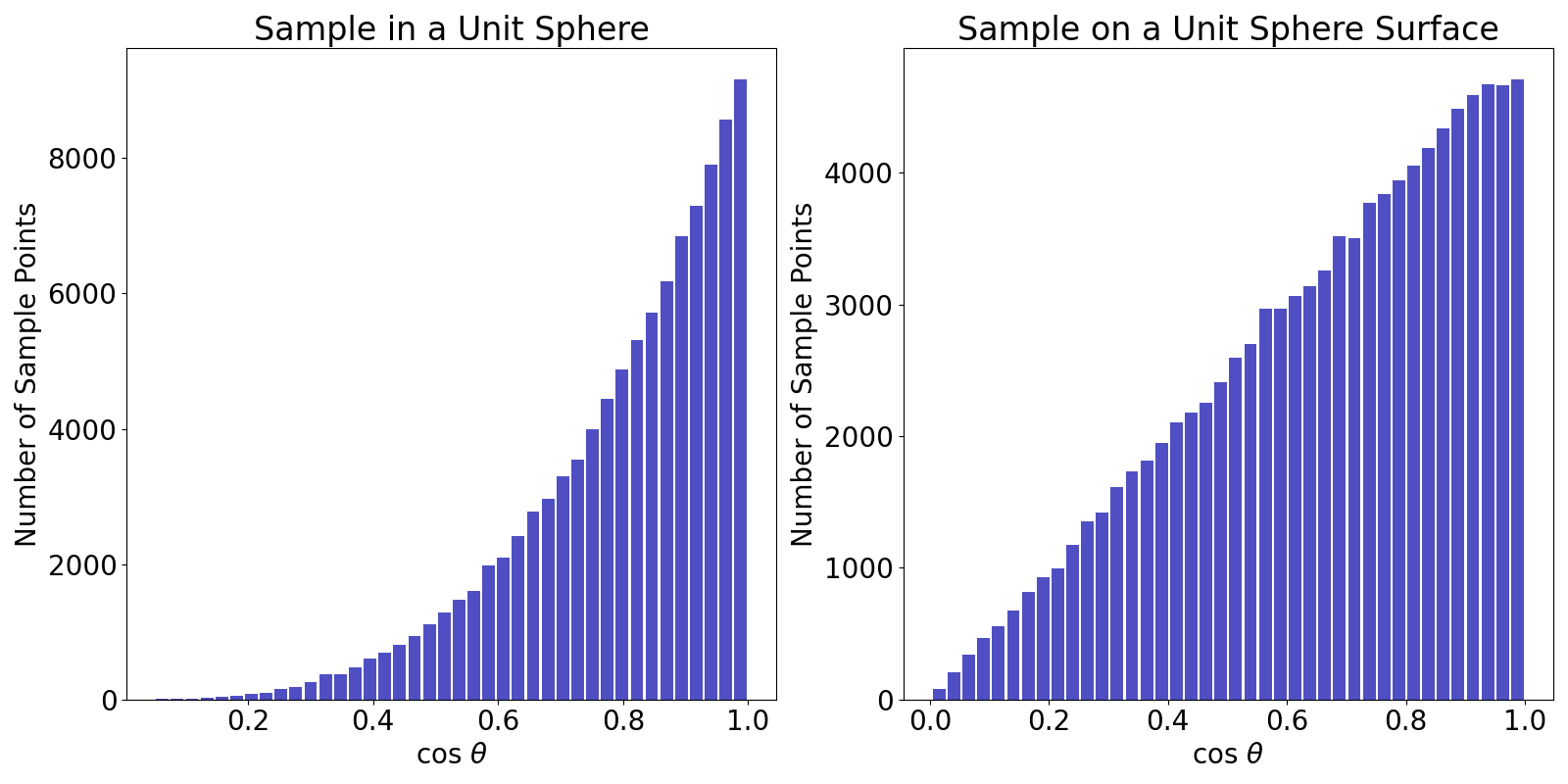
Sampling a Sphere
The rejection method: (Higher rejection rate for higher dimension problem (higher costs))
- Sample inside a uniform sphere:
- Sample on a uniform sphere: Sample inside a uniform sphere and project
Importance Sampling
- Sample inside a uniform sphere:
A
Alternative: uniformly sample a point on a uniform sphere centered at
 normalized
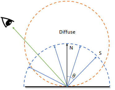
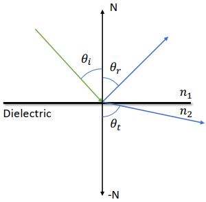
Reflection v.s. Refraction
Law of reflection:
Snell’s law (for refraction):
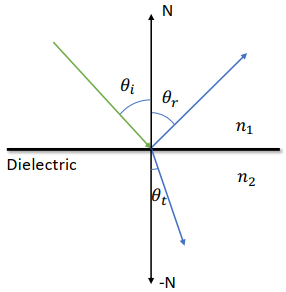
Total Reflection
Happens when
Snell’s law may fail to give
Reflection Coefficient R
At a steep angle => Reflection Coefficient
Refraction Coefficient
Fresnel’s Equation
S-polarization (perpendicular to)
P-polarization (parallel to)
For “natural light”:
Schlick’s Approximation
Material and angle
Path Tracing with R
xxxxxxxxxxdef scatter_on_a_dielectric_surface(I): sin_theta_i = -I.cross(N) theta_i = arcsin(sin_theta_i) if n1/n2*sin_theta_i > 1.0: return R # total internal reflection else: R_c = reflectance(theta_i, n1, n2) if random() <= R_c: return R # reflection (in = out) else: return T # refraction (Snell's law)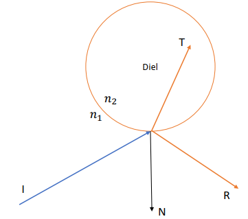
Recursion in Taichi
Call functions: temp var. -> storage in stack => higher pressure
Better solution -> using loops for tail-resursion
Optimization: Remain the fronter part of breaking loops; modify the tail-recursion part:
xxxxxxxxxx... ... ... else: brightness *= material.color / p_RR ray_o = P ray_dir = scatter(ray_dir, P, N) # the cos(theta) in DIFFUSE is hidden in the scatter function return color Anti-Aliasing
Zig-zag artifacts -> softening the edges
In this case we can use 4 times of random sampling -> anti-aliasing
Lecture 8 Deformable Simulation 01: Spatial and Temporal Discretization (21.11.16)
Laws of Physics
Equation of Motion
Define:
Linear ODE:
For linear materials,
Widely used for small deformation, such as physically based sound simulation (rigid bodies) and topology optimization
General Cases:
Integration in Time
Equation of Motion
Use
Explicit (forward) Euler Integration
Extremely fast, but increase the system enery gradually (leads to explode) -> seldom used => Symplectic Euler Integration
Symplectic Euler Integration
Also very fast. Update the velocity first -> momentum preserving, oscillating system Hamiltonian (could be unstable) -> Widely used in accuracy centric applications (astronomy simulation / molecular dynamics /…)
Implicit (backward) Euler Integration
Often expensive. Energy declines, damping the Hamitonian from the osscillating components. Often stable for large timesteps -> Widely used in performance-centric applications (game / MR / design / animation)
Integration in Space
Mass-Spring System
- Tessellate the mesh into a discrete one
- Aggregate the volume mass to vertices
- Link the mass-vertices with springs
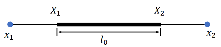
Deformation
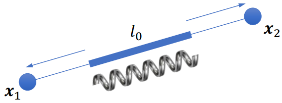
Spring current pose:
Spring current length:
Spring rest-length:
Deformation:
Deformation (Elastic) evergy (Huke’s Law):
Gradient:
Demo
Compute force
xxxxxxxxxx.kerneldef compute_gradient():# clear gradient for i in range(N_edges): grad[i] = ti.Vector([0, 0])
# gradient of elastic potential for i in range(N_edges): a, b = edges[i][0], edges[i][1] r = x[a]-x[b] l = r.norm() l0 = spring_length[i] k = YoungsModulus[None]*l0 # stiffness in Hooke's law gradient = k*(l-l0)*r/l grad[a] += gradient grad[b] += -gradientTime integration
xxxxxxxxxx# symplectic integrationacc = -grad[i]/m - ti.Vector([0.0, g])v[i] += dh*accx[i] += dh*v[i]Applications
Cloth sim / Hair sim
Not the best choice when sim continuum area/volume: Area/volume gets inverted without any penalty => Linear FEM
Constitutive Models
Deformation Map
A continuous model to describe deformation:
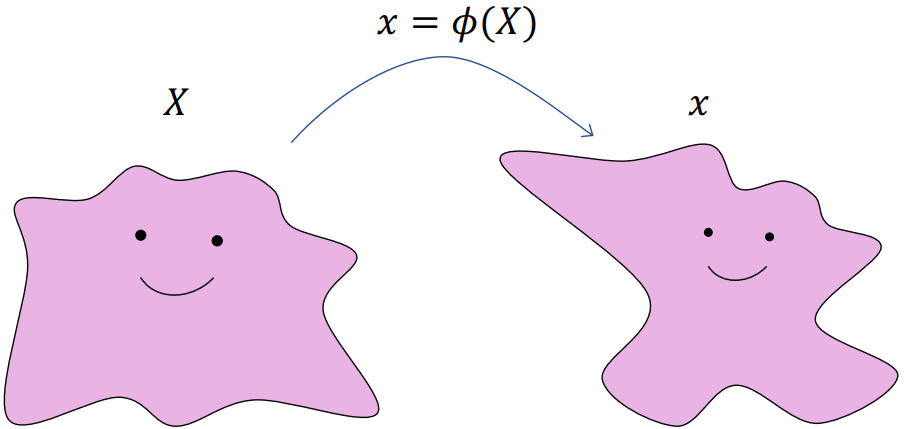
- Translation:
- Rotation:
- Scaling:
Generally: For
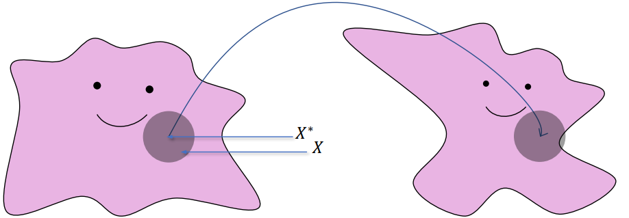
(
After approx, close to a translation in very small region:
=> A non-rigid deformation gradient shall end up with a non-zero deformation energy
Energy Density
- An energy density function at
- Energy density function should be translational invariant:
- We have
=> Deformation gradient is NOT the best quantity to describe deformation
Strain Tensor
Strain tensor:
- Descriptor of severity of deformation
Samples in different constitutive models:
- St. Venant-Kirchhoff model:
- Co-rotated linear model:
From energy density function to energy:
Linear Finite Element Method (FEM)
Linear FEM Energy
Continuous Space:
Discretized Space:
Find deformation gradient: Original pose (Uppercase) => Current pose
Find the gradient of
Chain rule: (Note:
1st Piola-Kirchhoff stress tensor for hyperelastic matrial:
Some 1st Piola-Kirchhoff stress tensors:
St. Venant-Kirchhoff model (StVK):
- Strain:
- Energy density:
- Strain:
Co-rotated Linear Model:
- Strain:
- Energy density:
- Strain:
Linear FEM
- Elastic energy:
- Gradient:
- Gradient of energy density:
For
-> Taichi: Autodiff
Demo
General Method:
Compute Energy
xxxxxxxxxx# gradient of elastic potentialfor i in range(N_triangles):Ds = compute_D(i)F = Ds@elements_Dm_inv[i]# co-rotated linear elasticityR = compute_R_2D(F)Eye = ti.Matrix.cols([[1.0, 0.0], [0.0, 1.0]])# first Piola-Kirchhoff tensorP = 2*LameMu[None]*(F-R) + LameLa[None]*((R.transpose())@F-Eye).trace()*R#assemble to gradientH = elements_V0[i] * P @ (elements_Dm_inv[i].transpose())a,b,c = triangles[i][0],triangles[i][1],triangles[i][2]gb = ti.Vector([H[0,0], H[1, 0]])gc = ti.Vector([H[0,1], H[1, 1]])ga = -gb-gcgrad[a] += gagrad[b] += gbgrad[c] += gcTime integration
xxxxxxxxxx# symplectic integrationacc = -grad[i]/m - ti.Vector([0.0, g])v[i] += dh*accx[i] += dh*v[i]With autodiff
Compute energy
xxxxxxxxxx.kerneldef compute_total_energy():for i in range(N_triangles):Ds = compute_D(i)F = Ds @ elements_Dm_inv[i]# co-rotated linear elasticityR = compute_R_2D(F)Eye = ti.Matrix.cols([[1.0, 0.0], [0.0, 1.0]])element_energy_density = LameMu[None]*((FR)@(F-R).transpose()).trace() + 0.5*LameLa[None]*(R.transpose()@F-Eye).trace()**2total_energy[None] += element_energy_density * elements_V0[i]Compute gradient
xxxxxxxxxxif using_auto_diff:total_energy[None]=0with ti.Tape(total_energy):compute_total_energy()else:compute_gradient() # use this funcTime integration
xxxxxxxxxx# symplectic integrationacc = -x.grad[i]/m - ti.Vector([0.0, g]) # this `x.grad` will be 2n*1 vector (same with compute_grad)v[i] += dh*accx[i] += dh*v[i]
Revisit Mass-spring System
- Deformation gradient:
- Deformation strain:
- Energy density:
- Energy:
Lecture 9 Deformable Simulation 02: The Implicit Integration Methods (21.11.23)
The Implicit Euler Integration
Time Step
In simulation: The time difference between the adjacent ticks on the temporal axis for the simulation:
v[i] += h * accx[i] += h * v[i]
In display: The time difference between two images displayed on the screen:
Sub-(time)-stepping:

The smaller
- For explicit integrations: too long time step may lead to explosion (as
- For implicit: usually converge for all
Numerical Recipes for Implicit Integrations
The Baraff and Witkin Style Solution
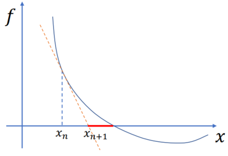
One iter of Newton’s Method, referred as semi-implicit
Goal: Solving
Assumption:
Algorithm: Non-linear -> Linear (
Let
Substitute this approx:
The solution is actually the location of
Reformulating the Implicit Euler Problem
To reduce the red part: add another step:
Integrating the nonlinear root finding problem over
Note: (Matrix Norm)
Minimization / Non-linear Root-finding:
Let
Then
For nonsingular
Convex Minimization of
The general descent method:

xxxxxxxxxxdef minimize_g(): x = x_0 while grad_g(x).norm() > EPSILON: Determine a descent dir: dx Line search: choose a stepsize: t > 0 Update: x = x + t * dxDetermine a descent dir:
Opt 1: Gradient Descent:
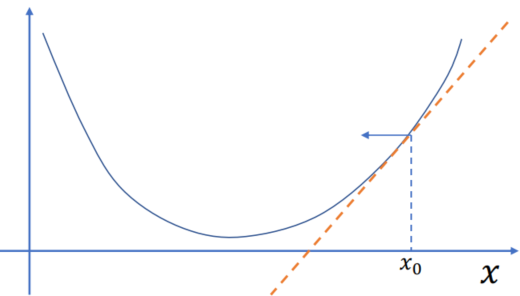
Opt 2: Newton’s Method:
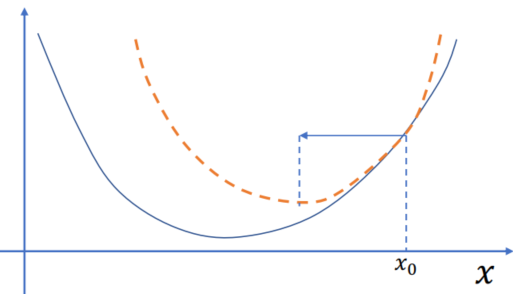
Find the step size:
Line search: choose a step size
Backtracking:
xxxxxxxxxxdef line_search():t = t_0while g(x) + alpha*t*grad_g(x).dot(dx) < g(x+t*dx):# this alpha indicates a line between the grad and the line w/ alpha = 0t = t * betareturn t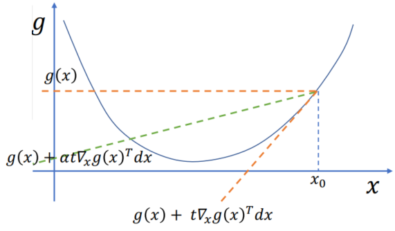
Problem
But most deformable bodies have non-convex energies: unsteady equilibrium.

Steps
Init guess:
While loop: while not converge:
Descent dir:
- Gradient:
- Hessian (Matrix):
- Gradient:
Line search: det the stepsize
Update:
Definiteness-fixed Newton’s Method
For general cases:
in Step 2 (while), After compute gradient dir and Hessian, add another substep:
- Fix Hessian to positive definite:
Definiteness-fix
Opt 1: Global Regularization
Init:
flag = False,reg = 1while not flag:flag,L = factorize(~H)Try to factorizereg = reg * 10
Opt 2: Local Regularization (in mass-spring system)
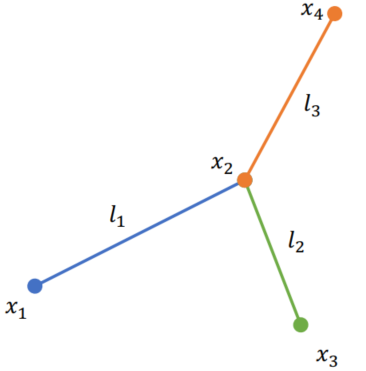
Has a sufficient condition:
After this definiteness-fix: (Newton’s)

Linear Solvers
Linear Solvers for
Direct solvers
Inversion:
Factorization (usually better especially for sparse matrices):
Interative solvers
- Stationary iterative linear solvers: Jacobi / Gauss-Seidel / SOR / Multigrid
- Krylov subspace methods: Conjugate Gradient (CG) / biCG / CR / MinRes / GMRes
Factorization
For
Solve
First solve
Then solve
For sparse matrices -> complexity not high; But not parallized (CPU backend only)
Current APIs:
[SparseMatrixBuilder] = ti.linalg.SparseMatrixBuilder()[SparseMatrix] = [SparseMatrixBuilder].build()[SparseMatrixSolver] = ti.linalg.SparseSolver(solver_type, ordering)[NumpyArray] = [SparseMastrixSolver].solve([Field])
Conjugate Gradient (CG) Method
Properties:
- Works for any symmetric positive definite matrix
- Guarantees to converge in
- Works amazingly good if the condition number
- Short codes
Demo: (Python scope - control flow)
xxxxxxxxxxdef conjugate_gradient(A, b, x): i = 0 r = b – A @ x d = r delta_new = r.dot(r) delta_0 = delta_new while i < i_max and delta_new/delta_0 > epsilon**2: q = A @ d # Matrix-Vector multiplication -> expensive alpha = delta_new / d.dot(q) # dot prod -> expensive x = x + alpha*d r = b - A @ x # r = r - alpha * q delta_old = delta_new delta_new = r.dot(r) beta = delta_new / delta_old d = r + beta * d i = i + 1 return xAccelerate the CG Method
Reduce the time of sparse-matrix-vector multiplication of
q = A @ d: (Piece-wise multiply)Use
@ti.kernel-> computing(Taichi enables thread local storage automatically for this reduction problem) (Taichi TLS / CUDA Reduction Guide)
Reduce the condition number of
The error (Upper bound)
Instead of solving
- Jacobi:
- Incomplete Cholesky:
- Multigrid
- Jacobi:
Lecture 10 Fluid Simulation 01: The Particle-based (Lagrangian) Methods (21.11.30)
Lagrangian Method = Particle-Based
Incompressible Fluid Dynamics
usually compressible for explosion / shock wave / … ; incompressible for slower dynamics
Forces for Incompressible Fluids

Incompressible Navier–Stokes Equations
The Navier-Stokes Equation (
The Spatial Derivative Operators
Gradient:
Divergence:
Curl:
Laplace:
Time Discretization
Operator Splitting
General Steps
Separate the N-S Eqn into 2 parts and use half the timestep to solve each part (Advection-Projection)
Step 1: Input
Step 2: Input
Time Integration
Given
Step 1: Advection / external and viscosity force integration
- Solve:
- Update:
- Solve:
Step 2: Projection / pressure solver (Poisson Solver)
- Solve:
- Update:
- Solve:
Step 3: Update position
- Update:
- Update:
Return
Integration with the Weakly Compressible (WC) Assumption
Storing the density

Time Integration
Symplectic Euler Integration: In this case step 1 and 2 can be combined since they are both explicit (no order diff)
Step 1: Advection / external and viscosity force integration
- Solve:
- Update:
- Solve:
Step 2: Projection / pressure solver (Use the current-point-evaluated
- Solve:
- Update:
- Solve:
Step 3: Update position
- Update:
- Update:
Return
Spatial Discretization (Lagrangian View)
- Previous knowledge using Lag. View: Mesh-based simulation (FEM)
- Today: Mesh-free simulation => a simular example: marine balls
Basic Idea
Cont. view -> Discrete view (using particles):
Time integration (Symplectic Euler):
But still need to evaluate
Smoothed Particle Hydrodynamics (SPH)
Dirac Delta
Trivial Indentity
The Dirac function only tends to infinity at 0 but equals to 0 otherwise. And its overall integral is 1.
Widen the Dirac Delta
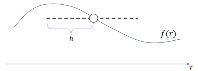
- Symmetric:
- Sum to unity:
- Compact support:
e.g.

Finite Probes: Summation
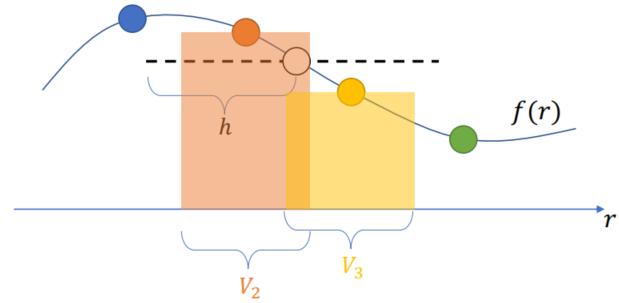
Smoother Kernel Function
Still use the summation:

Use a

Smoothed Particle Hydrodynamics (SPH)
Discretization
1D:
2D:
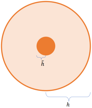
Par stored in every particles
Intrinsic quantities:
Time varying quantities:
Evaluate 2D fields using the SP

SPH Spatial Derivatives
The operators will affect only on the kernel func (
Improving Approximations for Spatial Derivatives
Let

Anti-symmetric Form
Better for projection / divergence / …
=> Since
- Or equivalently:
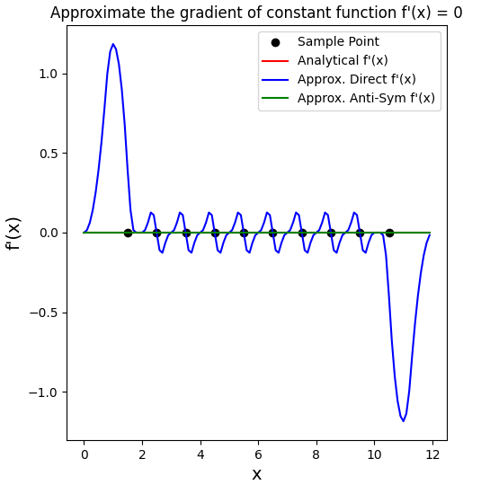
Symmetric Form
Better for forces
A more gen case:
Special Case: when
Implementation Details (WCSPH)
Simulation Pipeline
For i in particles:
Search for neighbors j -> Apply the support radius

For i in particles:
Sample the
- Desity:
- Viscosity:
- Pressure Gradient:
- Desity:
Compute
For i in particles (Symplectic Euler)
Update
Update
Boundary Conditions

Problems of Boundaries
Insufficient samples
Free Surface: lower density and pressure => Generate outward pressure
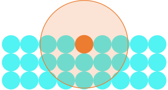
-> Sol: Clamp the negative pressure (everywhere),
Solid Boundary: lower density and pressure => Fluid leakage (outbound velocity)
-> Sol:
for leakage:
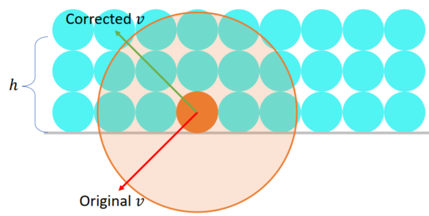
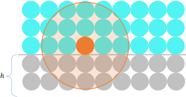
- Refect the outbound veclocity when close to boundary
- Pad a layer of SP underneath the boundaries:
Neighbor Search
Navie search:
=> Use background grid: Common grid size =
(Each neighbor search takes 9 grids in 2D and 27 grids in 3D)
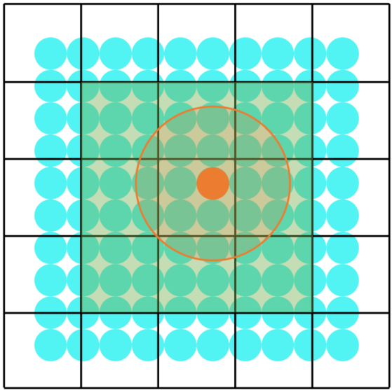
Lecture 11 Fluid Simulation 02: The Grid-based (Eulerian) Methods (21.12.6)
N-S Equations and Their Time Integration
Operator Splitting
A toy example:
Integrate
(for some quantity ) => Theoretical sol: Operator Splitting:
;
Operation Splitting for N-S Eqn
(
One Numerical Time-Stepping for N-S Eqn
Given
Step 1: Advection: (Solve intuitive formula) => in Lag (trivial), in Euler (not trivial)
Step 2: Applying forces: (The term of viscosity could be neglected when simulate gas; gravity can be neglected when the gas has similar density as air)
Step 3: Projection: (Solve for pressure and ensure divergence free)
Return
From the Lagrangian View to the Eulerian View
In Eulerian grids: Need to record: grid index / velocity / density / temperature / grid size / …
Lagrangian: Dynamic markers
- Pros: Advection (Quantity preservation) / Boundary Condition (Conformal discretization) / Coupling with solids
- Cons: Spatial derivative / High spatial discretization error / Neigh search / Unbounded distortion / Explicit collision handling
Eulerian: Static markers
- (On the opposite side of Lagrangian)
Spatial Derivatives Using Finite Difference
Spatial derivative: The dimensions can be decoupled when computing the spatial derivatives due to the structural grid
To compute
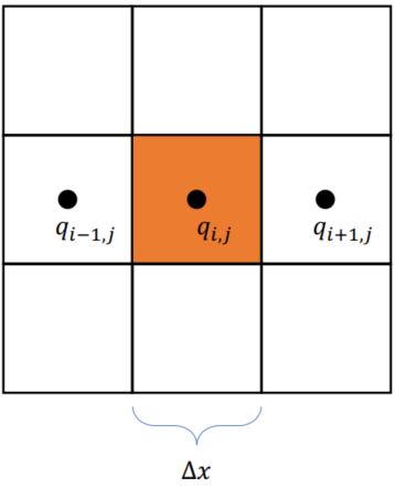
Forward difference:
Central difference:
Problem of the central difference: Non-constant functions are able to register a zero spatial derivative
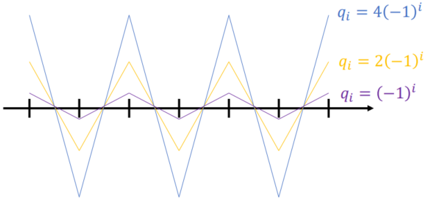
Central difference with a “staggered” grid:
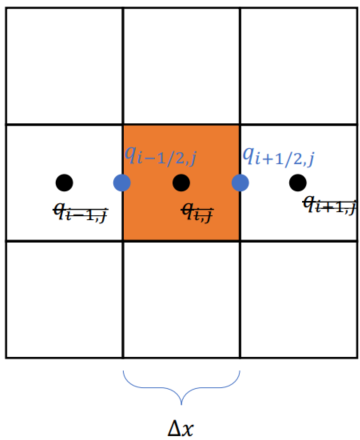
Usually store the velocity using the staggered fashion (edges); and store the other (scalar) quantities in the grid centers (e.g. temperature / density / pressure)
MAC (Marker-and-Cell) grid
Staggered Grid
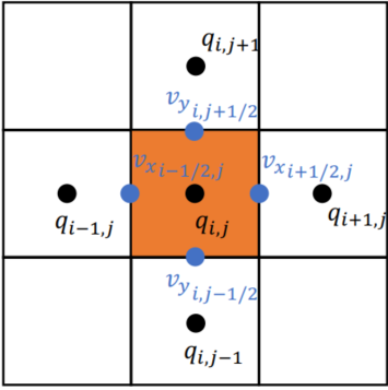
For a row x col grid (3x3) storage:
- Temperature (or other scalars): 9
- velocity
Staggered Grid in Stokes Theorem
Exterior calculus
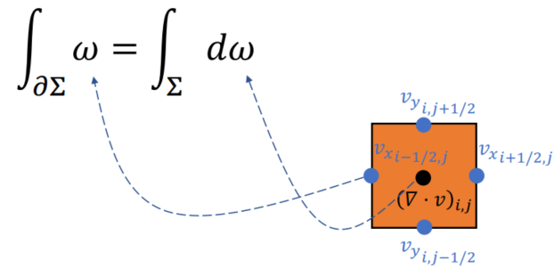
Advection
Material Derivative
Material Derivative of Vectors
If
For velocity (self-advection)
Quantity Advection
In Eulerian view, quantities flow with the velocity field for
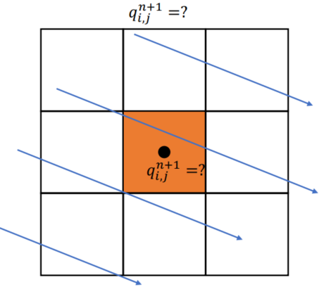
Attempt 1: Finite Difference
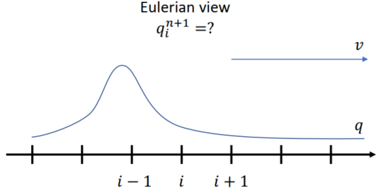
1-D Advection: Unconditionally Unstable w/. FTCS
Attempt 2: Semi-Lagrangian
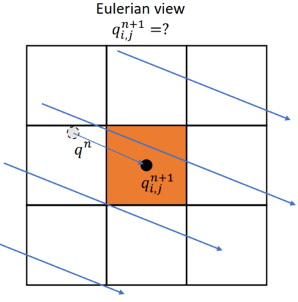
To find value of
Usually use Bilinear interpolation in 2D:
1-D Advection: Unconditionally Stable (The peak will stably move forward) => Required
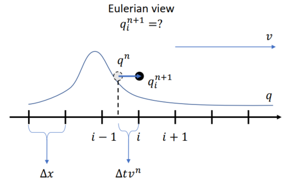
Assuming:
Problems:
Increase the numerical dissipation/viscosity
=> Some better schemes with less dissipation:
Sharper Interpolation (Cubic Hermit spline interpolation)
Better error correction schemes
- MacCormack Method
- Back and Forth Error Compensation and Correction (BFECC)
Backtracked “particle” out-of-boundary:
Simplest sol: Take the value of the boundary
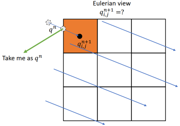
Projection
Poisson’s Equation
Possion’s Problem
Want to solve
Use finite difference again:
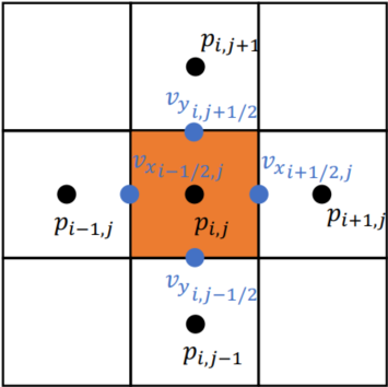
The condition will not be divergence free => becomes
Another way to achieve Possion’s problem:
- Want:
- Discretize the pressure equation in time:
- Apply divergence operator
Pressure Solve
For every grid: One unknown
For every grid: One equation:
Require only a linear solver:
All pressure are solved than to update velocity:
But velocity values are more than pressure values => introducing boundary conditions
Boundary Conditions
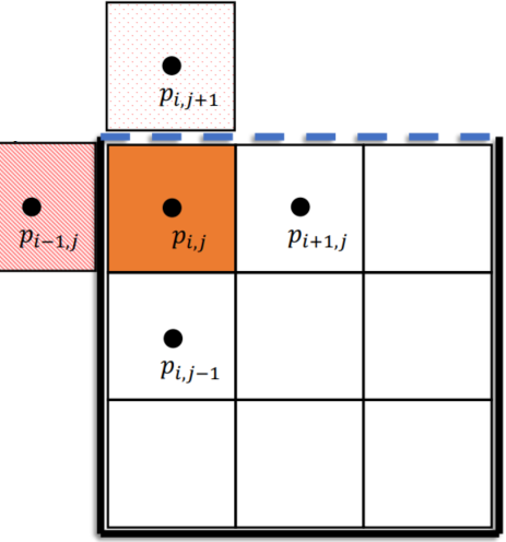
Free Surface (Dirichlet)
Solid Wall (Neumann)
For solid grids:
Boundary Conditions in Possion’s Problem
Dirichlet:
Neumann:
The Possion’s equation with boundaries:
To solve