GAMES101 - Overview of Computer Graphics
Lecturer: Lingqi Yan
Lecture Videos | Course Site | HW Site
Linear Algebra (Lec. 2)
Cross Product
Check whether a point
Check whether a point
(Corner case:
Matrices
Product can be operated:
- Dot Product:
- Cross Product:
Transformation (Lec. 3-4)
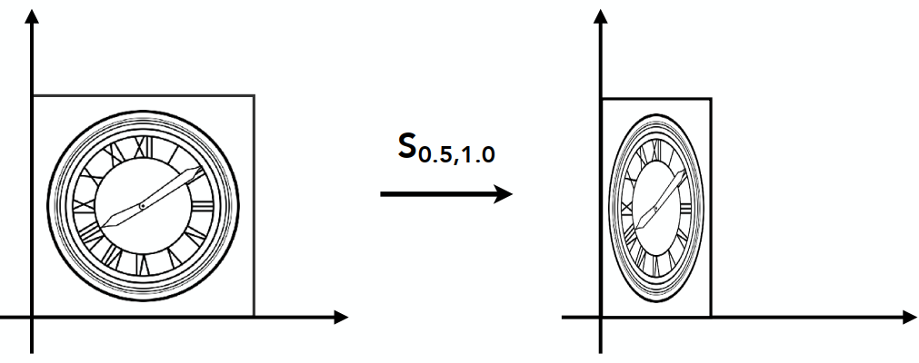
Transformation
Scale Matrix: Ratio s:
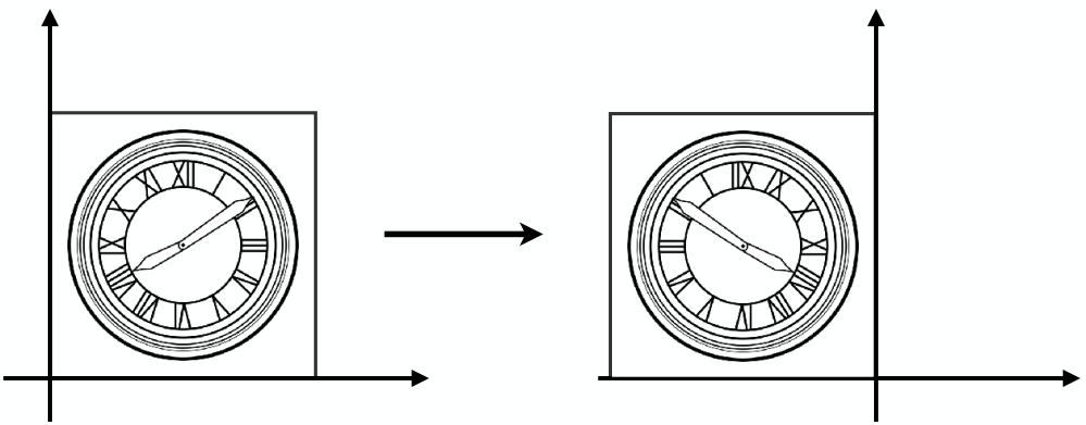
Reflection Matrix:
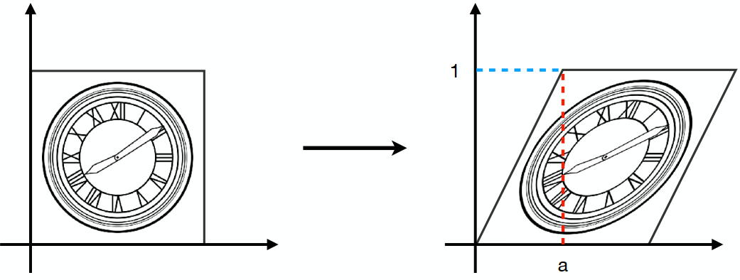
Shear Matrix:
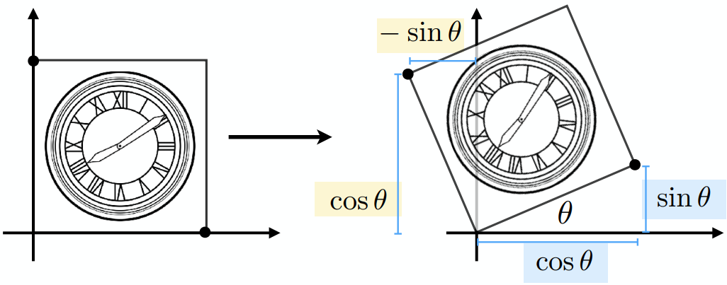
Rotate (2D) around (0, 0), counter-clock
Translation (Not linear transformation)
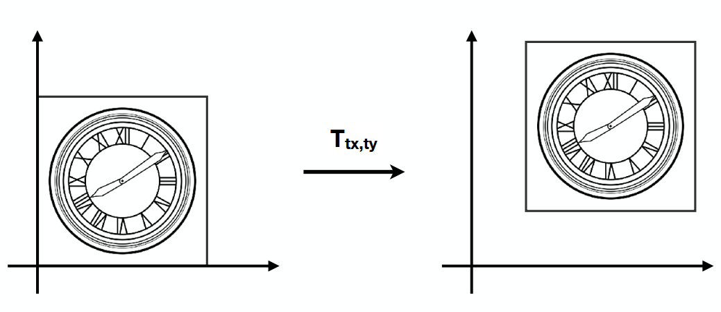
Homogeneous Coordinates
(Add a third coordinate - w-coordinate)
2D point = (x, y, 1)T
2D vector = (x, y, 0)T (平移不变性:Direction and magnitude only)
Vector + Vector = Vector (0 + 0)
Point - Point = Vector (1 - 1)
Point + Vector = Point (0 + 1)
Point + Point = ?? (1 + 1) (Actually, Mid point)
Affine Transformation
仿射
Affine map = linear map + translation
Inverse Transformation
Composite Transform
Transformation Ordering Matters
Notice that the matrices are applied right to left(无交换律 但有结合律)
e.g.
Pre-multiply n matrices to obtain a single matrix representing combined transform (for performance)
Example: (Decomposing)
Rotate around point C:
Representation:
3D Transformation
3D point = (x, y, z, 1)T
3D vector = (x, y, z, 0)T
~ (x/w, y/w, z/w)
Homogeneous Coordinates
Order: Linear transformation first, then translation(先线性变换,再平移)
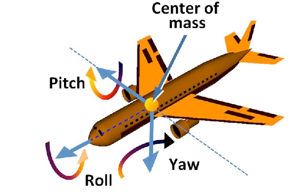
Rotate around Axis
x-axis:
y-axis:
Compose any 3D Rotations from Rx, Ry, Rz
Rodrigues’ Rotation Formula: By angle
Viewing Transformations
View / Camera Transformation(视图变换)
MVP: Model-View Projection
(Model transformation: placing objects; View transformation: placing camera; Projection transformation)
Define camera first:
- Position:
- Look-at / gaze direction:
- Up direction:
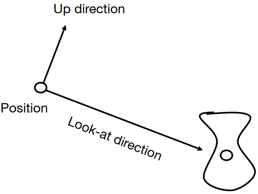
Key Observation: If the camera and all objects move together, the “photo” will be the same => Transform to: the origin with up @ Y, look @ -Z
Transformation Matrix
(Also known as model-view transformation)
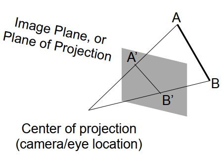
Projection Transformation
Orthographic Projection
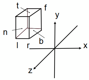
Camera @ 0, Up @ Y, Look @ -Z. Translate & Scale the resulting rectangle to [-1, 1]2
(Looking at / along -Z is making near and far not intuitive (n > f). OpenGL uses left hand coordinates)
In general, map a cuboid [l, r] x [b, t] x [f, n] to canonical cube [-1, 1]3
Transformation Matrix:
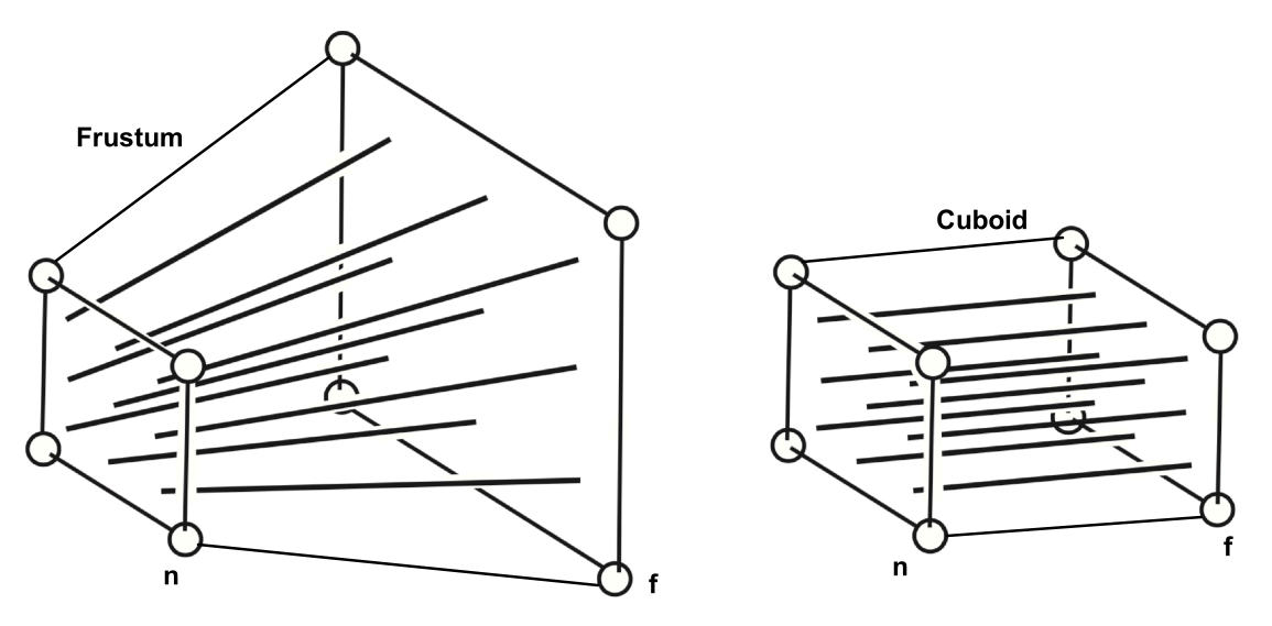
Perspective Projection (Most common)
 (Not parallel)
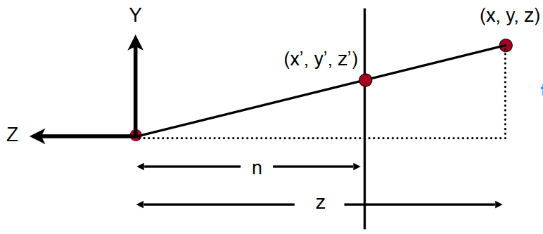 (Similar triangle
Process: Frustum(视锥)- (n - n, f - f) - Cuboid - Orthographic Proj. (Mo)
(近平面不变,远平面中心不变)
In homogeneous coordinates:
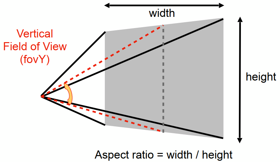
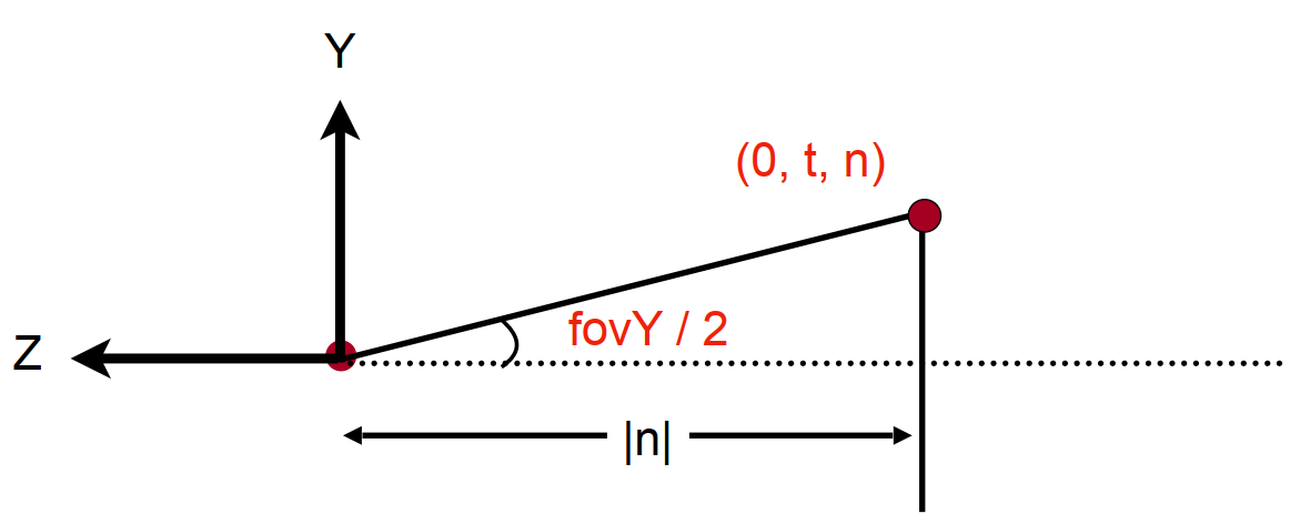
Vertical Field of View (fovY) (Assuming symmetry: l = -r; b = -t)
Rasterization (Lec. 5-7)
Rasterize
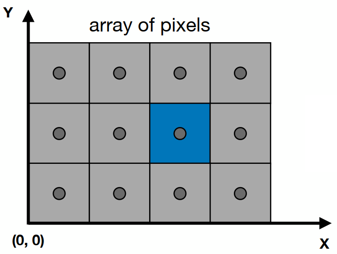
Rasterize = Draw onto the screen
Define Screen Space: Pixel: (0, 0) - (Width - 1, Height - 1)(均匀小方块); Centered @ (x + 0.5, y + 0.5) (Irrelavent to z)
Sampling (Approximate a Triangle)
Rasterization as 2D sampling
For triangles, each pixel is whether inside / outside should be checked.
xxxxxxxxxxfor (int x = 0; x < xmax; ++x) for (int y = 0; y < ymax; ++y) image[x][y] = inside(tri, x + 0.5, y + 0.5);Evaluating inside(tri, x, y)
3 cross products:
(Want: All required points (pixels) inside the triangle)
Edge cases: covered by both tri. 1 and 2: Not process / specific
Instead of checking all pixels on the screen, using incremental triangle traversal / a bouding box (AABB) can sometimes be faster
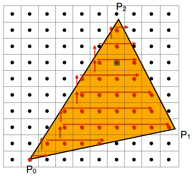 Suitable for thin and rotated triangles
Artifacts
(Error / Mistakes / Inaccuracies)
Jaggies (Too low sampling rate) / Noire / Wagon wheel effect (Signal changing too fast for sampling)
Idea: Blur - Sample
Frequency Domain
In freq. domain:
Fourier Transform:
(Higher freq. needs faster sampling. Or samples erroneously a low freq. signal)
Filtering: Getting rid of certain freq. contents (high / low / band / ...)
Filter out high freq. (Blur) - Low pass filter (e.g. Box function)
Theorem: Spatial domain · Filter (Convolution Kernel) = ...
Fourier domain
Convolution(卷积): (加权平均滤波器)Product in spatial domain = Convolution in frequency domain
Wider Kernal = Lower Frequency (Blurer)
Sampling = Repeating Frequency Contents
Aliasing = Mixing freq. contents (sampling too slow)
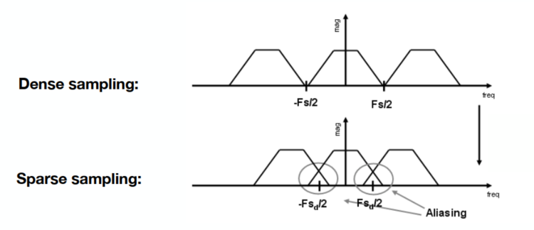
Reduction: Increasing sampling rate; Antialiasing (Blur - Sample, Make F contents "narrower")
Antialiasing = Limiting, then repeating

Solution: Convolve
Antialiasing Techniques
MSAA (Multisample Antialiasing)
By supersampling (same effects as blur, then sampling) (1 pixel -> 2x2 / 4x4 & Average)
Cost: Increase the computation work (4x4 = 16 times) - Key pixel distribution
FXAA (Fast Approximation AA)
后期处理降锯齿,使用边界
TAA (Temporal AA)
Use the previous one frame for AA
Super Resolution (DLSS - Deep Learning Supersampling)
Visibility / Occlusion
Z (Depth) Buffering
深度缓存
Point Algorithm(由远到近 - 不好处理相互重叠的关系)
Z-buffer: Frame buffer for color values; z-buffer for depth (Smaller z - closer (darker); Larger z - farther (lighter))
Algorithm during Rasterization
xxxxxxxxxxfor (each triangle T) for (each sample (x, y, z) in T) if (z < zbuffer[x, y]) // Closest sample so far (是否更新该像素,判断 z) framebuffer[x, y] = rgb; // Update color zbuffer[x, y] = z; // Update depth (相同的可更可不更 - 可能为抖动) else ; // Do nothingComplexity: O(n)
For n triangles, only check. No other relativity.
Order doesn't matter
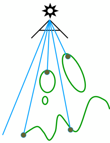
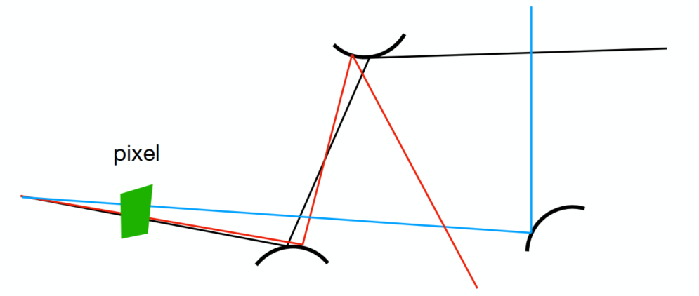
Supplement: Shadow Mapping
After Lec. 12
An image-space algorithm, widely used for early animations and every 3D video game
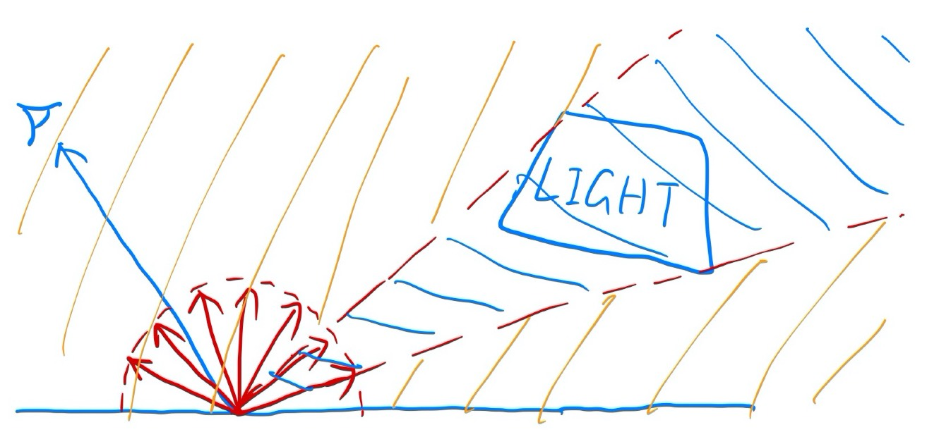
Key idea: The point not in shadow must be seen both by the light and the camera
Hard shadow: Use 0 & 1 only to represent in shadow or not
(between 0 and 1 -> soft shadow: by multiple light sources / source size)
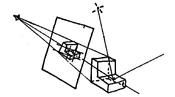
Approaches
Pass 1: Render from light (Rasterize the view with the light source)
Depth image from light source
Pass 2A: Render from eye
Standard image with depth from eye
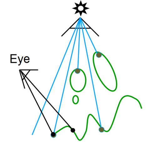
Pass 2B: Project to light
Project visible points in eye view back to light source
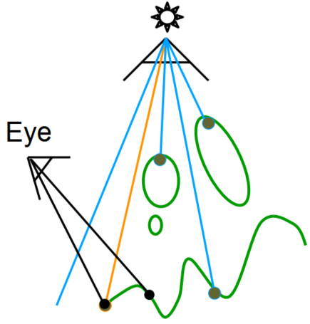
Orange line: (Reprojected) depths match for light and eye. VISIBLE
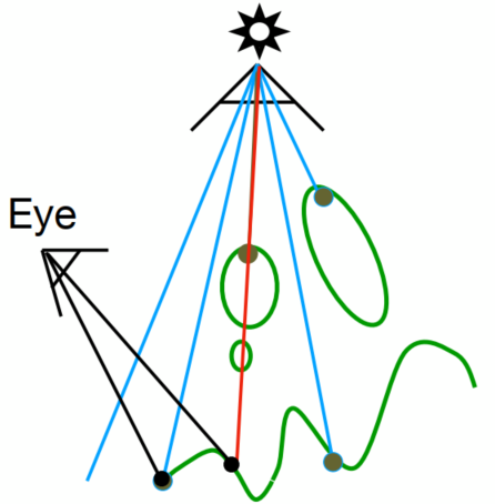
Red line: (Reprojected) depths from light and eye are not the same. BLOCKED!!
Problems with Shadow Maps
- Hard shadows (point lights only)
- Quality dep on shadow map resolution (gen problem with image-based techniques)
- Involves equality comparison of floating point depth values means issues of scales / bias / tolerance
Shading (Lec. 7-10)
Apply a material to an object
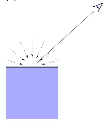
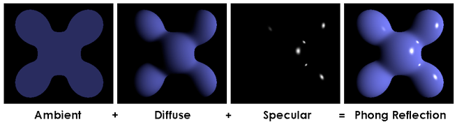
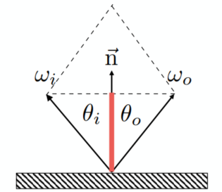
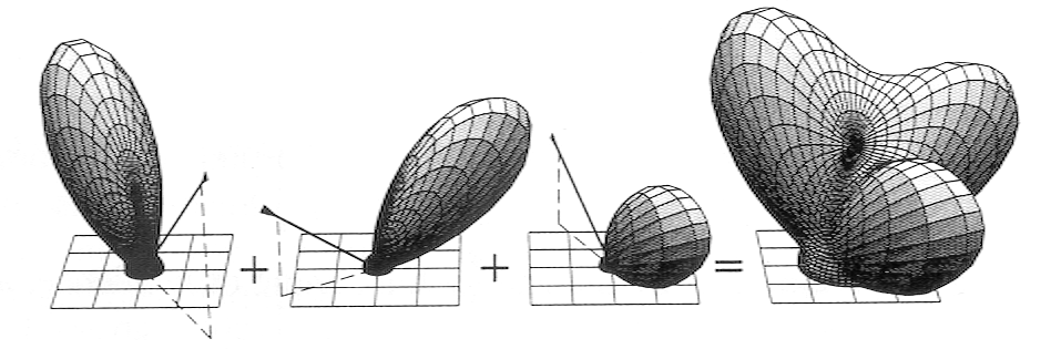
Shading Model (Blinn-Phong Reflectance Model)
Light reflected towards camera.
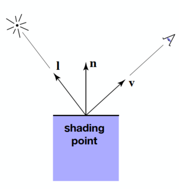
Viewer direction, v; Surface normal, n; Light direction, l (for each of many lights); Surface parameters (color, shininess, …)
Shading is local - No shadows will be generated
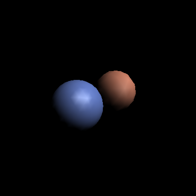
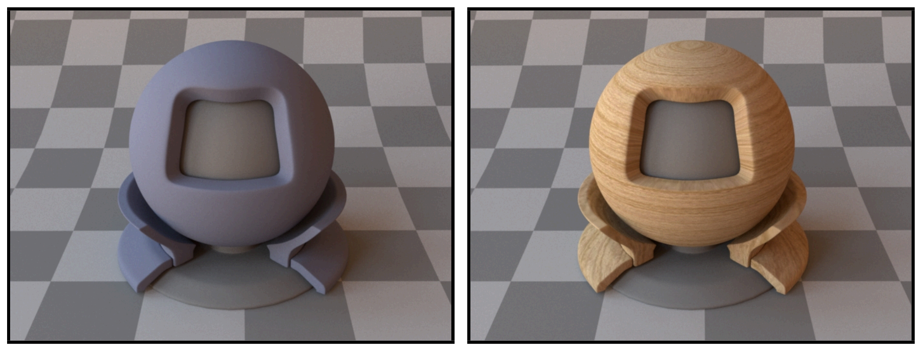
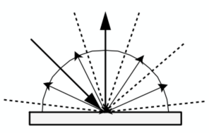
Diffuse Reflection
Light is scattered uniformly in all directions (Surface color is the same for all viewing direction)
Light Falloff (Beer Lambert's Law)
Lambertian (Diffuse) Shading
Shading independent of view direction
(
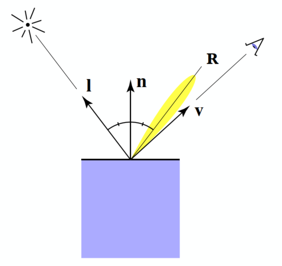
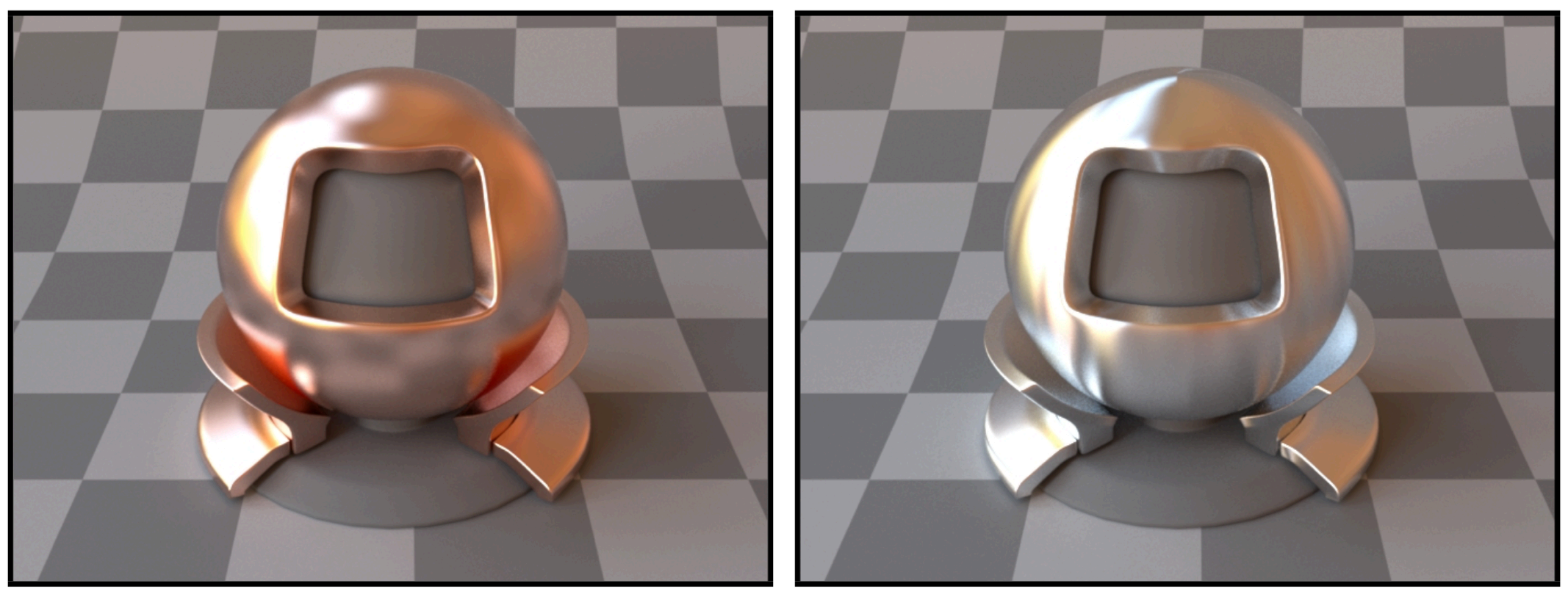
Specular
Intensity depends on view direction (Bright near mirror reflection direction)
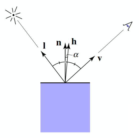
(
(Only use
Ambient
Not depend on anything
Fake approximation
Summary
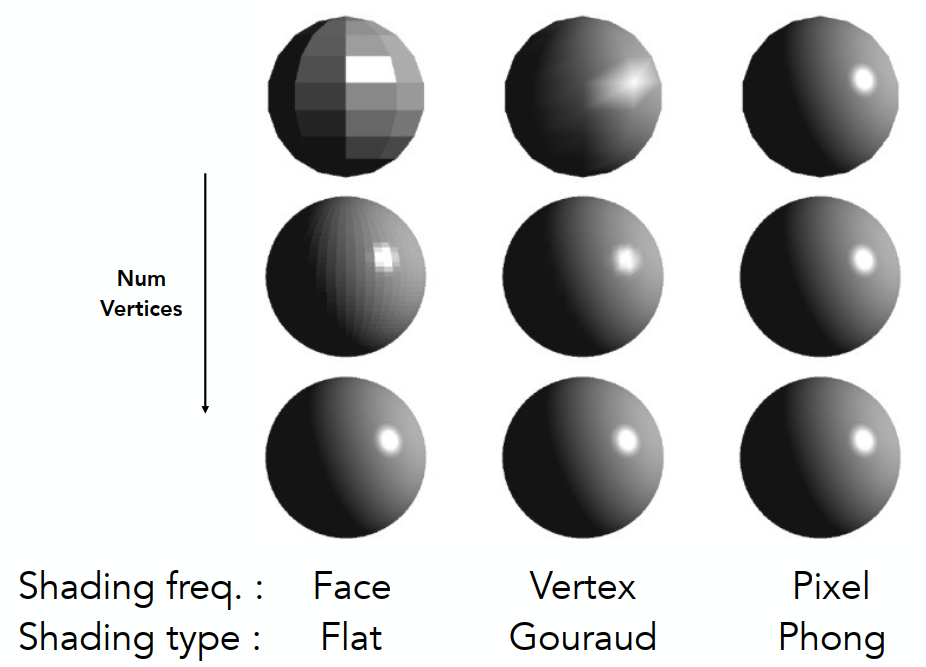
Shading Frequencies
(Face / Vertex / Pixel)
Shading Methods
- Shade each triangle (flat shading) - Not good for smooth surface
- Shade each vertex (Gouraud shading) - Interporate colors from vertices
- Shade each pixel (Phong shading) - Full shading model each pixel (Not the Blinn-Phong Reflectance Model)


Pre-Vertex Normal Vectors
Vertex normal - Average surrounding face normals
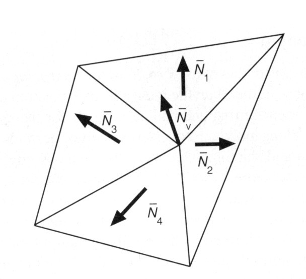
~ Barycentric interpolation of vertex normals (Need to normalize)
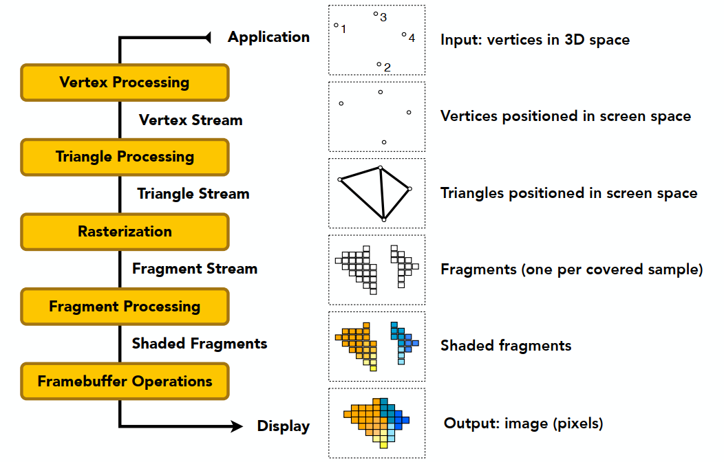
Graphics (Real-time Rendering) Pipeline
~ GPU
- Input: Model, View, Projection transforms
- Rasterization: Sampling triangle coverage
- Fragment Processing: Z-Buffering visibility test / Shading / Texture mapping
Texture Mapping
纹理映射 - UV ((u,v) coordinate) (
Barycentric Coordinates
Interpolation Access Triangles
Specific values @ vertices / smoothly varing across triangles
Barycentric Coordinates
A coordinate system for triangles
The barycentric coordinate of
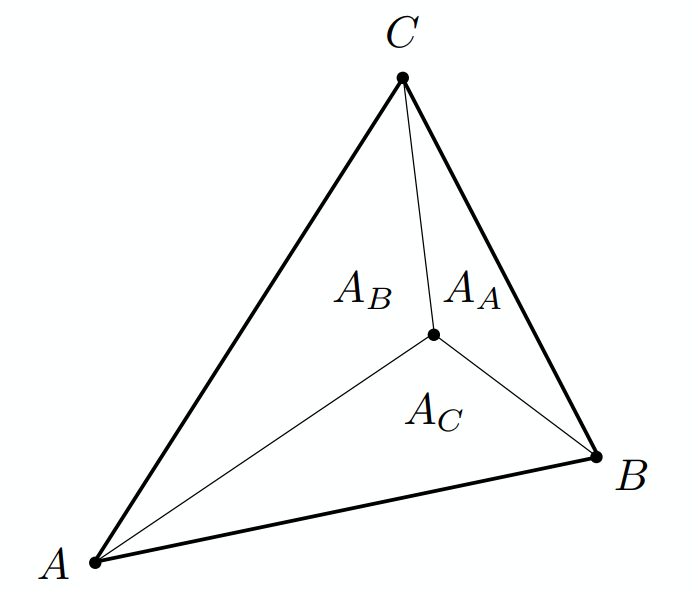
Geometric viewpoint — proportional areas:
Centroid:
Express any point:
Color interpolation for every point: linear interpolation
Disadvantage: Not invariant under projection (depth matters)
(3D - Use 3D interpolation OK; 2D - rather than use projection)
Apply: Diffuse Color
xxxxxxxxxxfor each rasterized screen sample (x,y) // Usually a pixel center (u,v) = evaluate texture coordinate at (x,y) // Applying Barycentric coordinates texcolor = texture.sample(u,v); set sample’s color to texcolor; // Usually diffuse kd (Blinn-Phong)Texture Magnification (AA)
(used for insufficient resolution)
Texel: A pixel on a texture(纹理元素 / 纹素)
Easy Cases
- Nearest
- Bilinear (Interpolation) - Pretty good results at reasonable costs
- Bicubic (Interpolation) - Instead of 4 points (bilinear), using 16 (4x4) points for 1 lerp
Bilinear Magnification
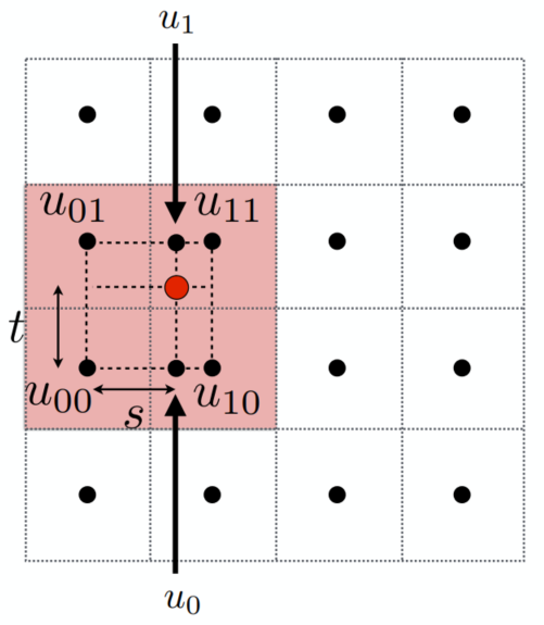
- Linear Interpolation (1D):
- Helper Lerps:
- Final Vertical Lerp:
Lerp - Linear Interpolation
Hard Cases
Problem of point sampling textures
(can be solved by supersampling but costly)
Near: Jaggies (Minification / Downsampling for too high resolution) ; Far: Moire (Upsampling)
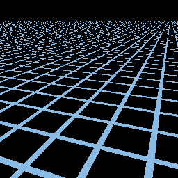
Mipmap
Allowing (fast, approx., square) range queries
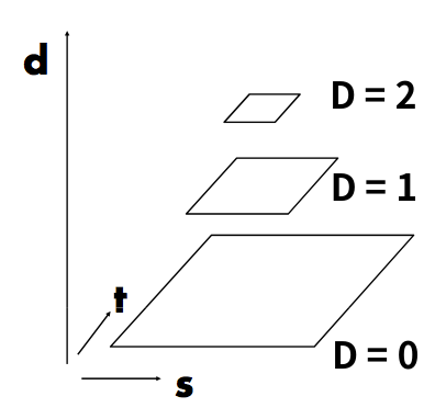
(Image Pyramid) "Mip Hierachy": level = D
Estimate texture footprint using texture coordinates of neighboring screen samples
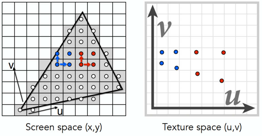
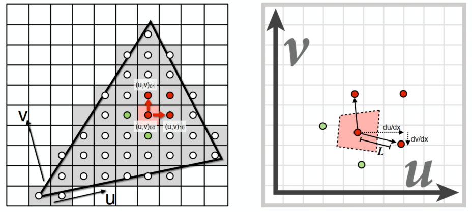 层查询 - 后者为选择较大 L 是近似(UV)
Near - range quires in low D level Mipmap; Far - high D level
If want more continuous results: interpolation between levels
Trilinear Interpolation
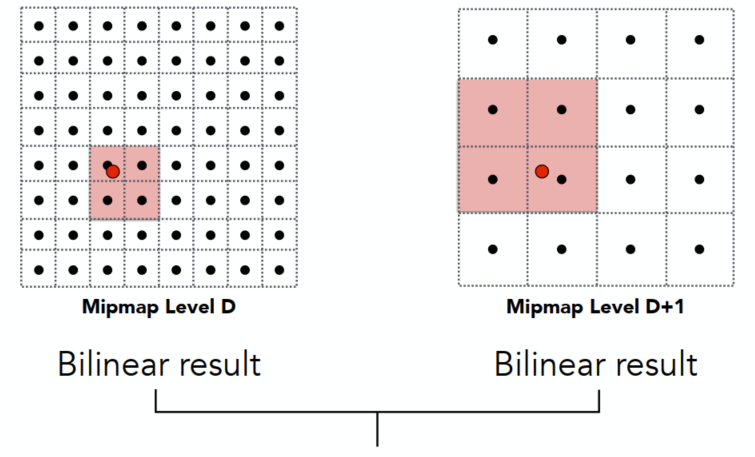
Linear interpolation (lerp) based on continuous D value
Limitations
In far and complex region - Overblur (box)
- Anisotropic filtering(各向异性过滤): look up axis-aligned rectangular zones(长方形区域搜寻), but still have problems in diagonal footprints - Ripmap (need graphics memory, doesn't need high flops x3)
- EWA filtering (Time computing costs): use multiple look ups / weighted average. able to handle irregular footprints
Applications of Textures
Environmental Map
Environmental Map: 有光从各个方向进入眼睛,所有光都有对应,用纹理映射环境光
不记录深度,都认为是无限远
Environmental Lighting: 环境光记录于球面 - 渲染时展开
Spherical EM (Problem: Prone to distortion (top and bottom))
Cube Map: A vector maps to cube point along that direction (6 square texture maps) - Less distortion but need direction for face computations
Right face has
Textures Affecting Shading
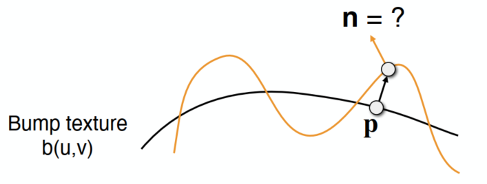
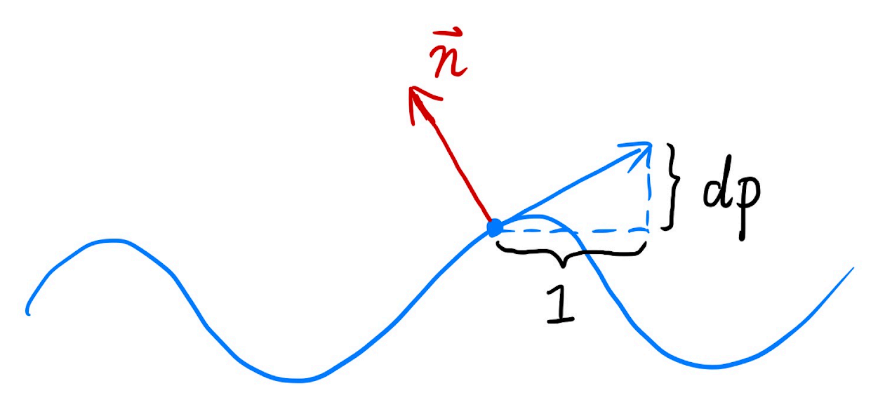
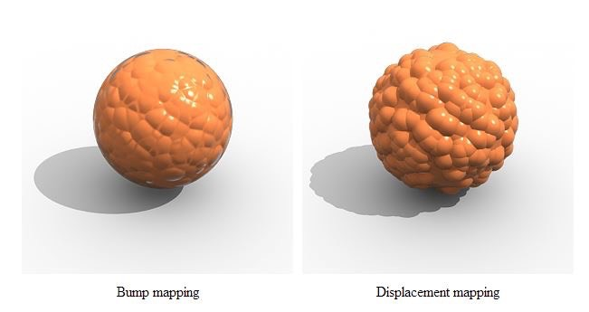
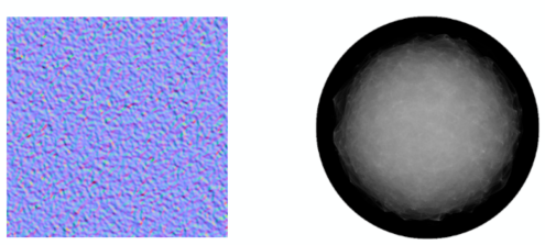
Bump / Normal Mapping
Adding surface details without adding more triangles (Perturb surface normal per pixel)
未改变几何 - 产生凹凸错觉
Perturb the nromal (in flatland)
Original surface normal:
Derivative @ p:
Perturbed normal:
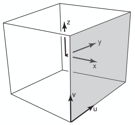
Perturb the normal (in 3D) (local coordinates)
- Original surface normal:
- Derivatives @ p:
- Perturbed normal:
- Original surface normal:
Displacement Mapping
Uses the same texture as in bumping mapping, but actually moves vertices
- 3D Procedural Noise + Solid Modeling
- Provide Precomputed Shading
- 3D Texture and Volume Rendering
Geometry (Lec. 10-12)
Representing Ways
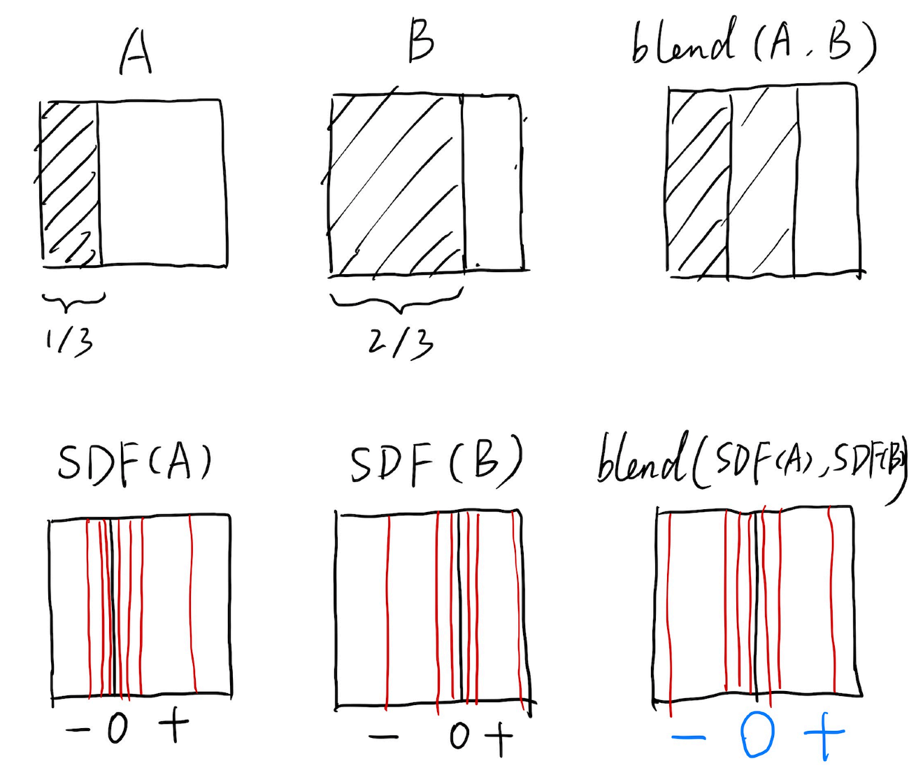
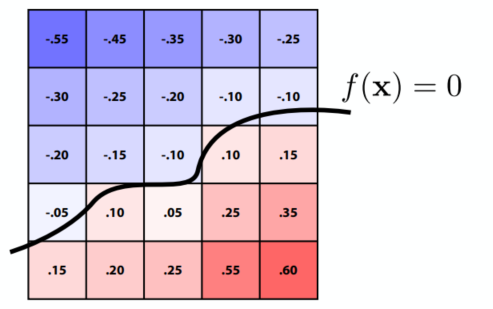
Implicit: algebraic surface / level sets(等高线法)/ constructive solid geometry (Boolean) / distance functions / fractal ...
(Don’t tell exact positions,tell spe. relationships. e.g. sphere:
Hard for sampling but easy for test in / outside
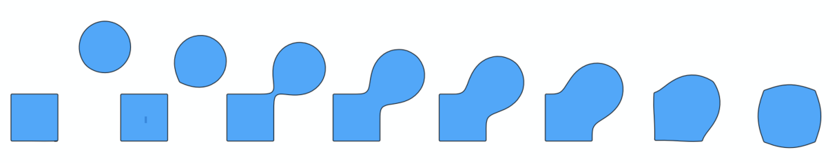
Distance functions:
Level Set: (CT / MRI)
Explicit: point cloud / polygon-mesh (.obj) / subdivision / NURBS / ...
(Generally,
Hard to test in / outside but easy to sample
Curves
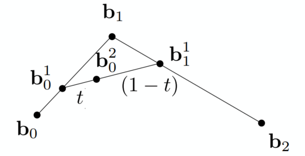
Bézier Curves (Explicit)
3 pt. - quadratic Bézier
Connect
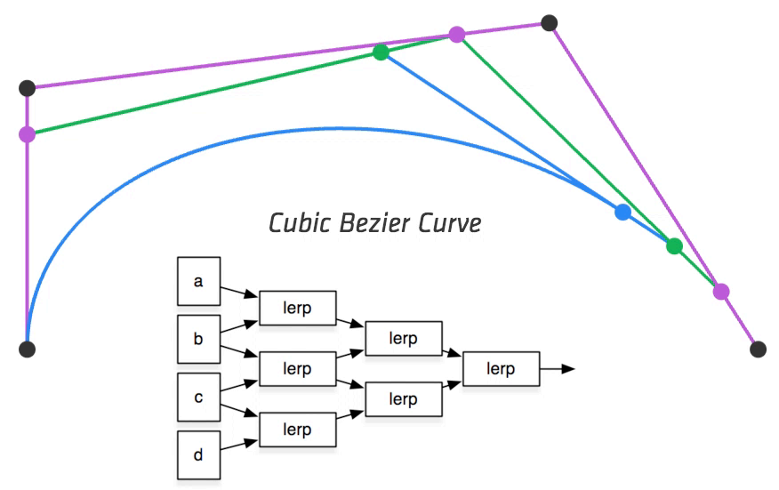
4 pt. - cubic Bézier
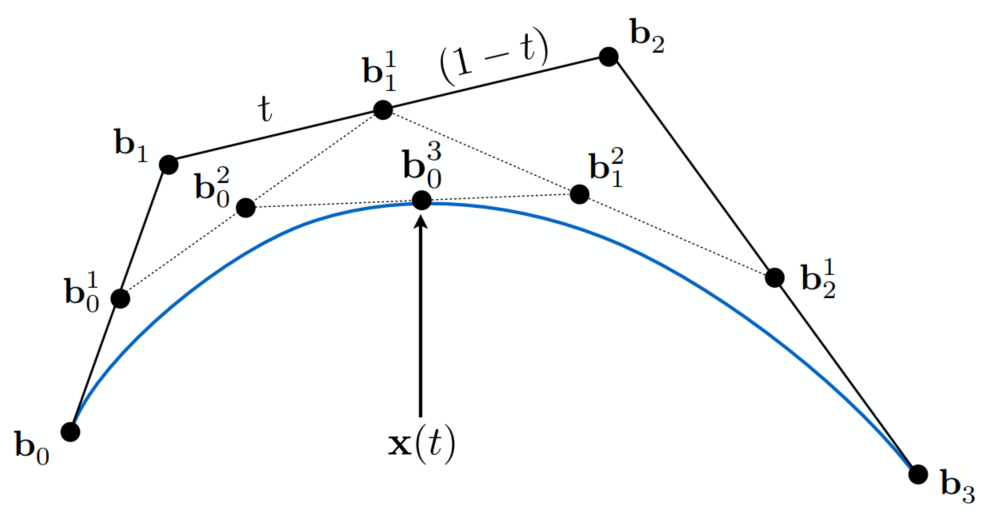
(De Casteljau’s Algorithm)
Evaluating Bézier Curves
Algebraic Formula
Bernstein form of a Bézier curve of order n:
(
where Bernstein polynomials:
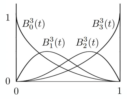
At anywhere, sum of
B-Splines
Could be adjusted partially
For C2 cont. -> NURBS (Non-Uniform Rational B-Splines)
Surfaces
- Bicubic Bézier: 4x4 array -> surface
- Mesh Operations: subdivision / simplification / regularization
Bézier Surfaces
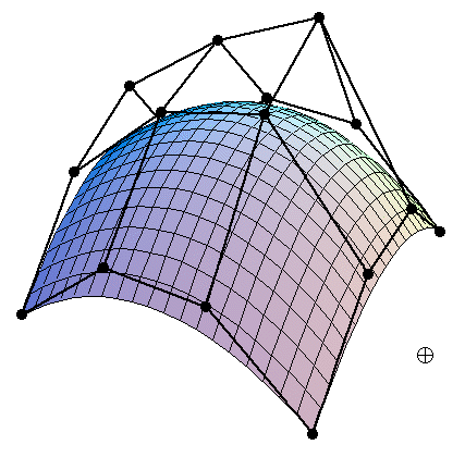
Extend Bézier curves to surfaces
Bicubic Bézier Surface Patch (4x4 array of control points)
Evaluating Surface Position for Parameters (u,v)
For bicubic Bézier surface patch:
Input: 4x4 control points; Output: 2D surface parameterized by
Method: Separable 1D de Casteljau Algorithm
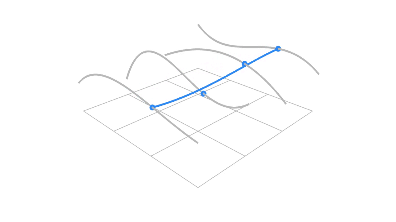
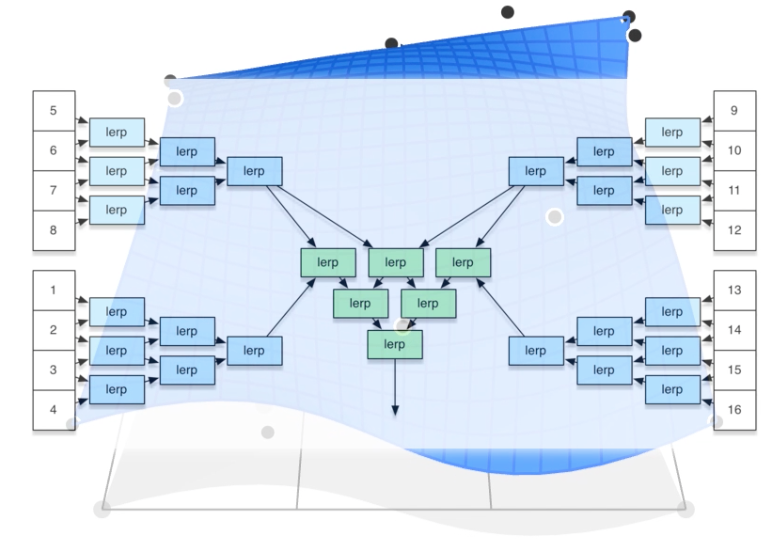
(u,v)-separable application of de Casteljau algorithm:
- Use de Casteljau to evaluate point u on each of the 4 curves in u -> gives 4 control points for “moving” the Bézier curve
- Use 1D de Casteljau to evaluate point v on the “moving” curve
Mesh Operations: Geometry Processing
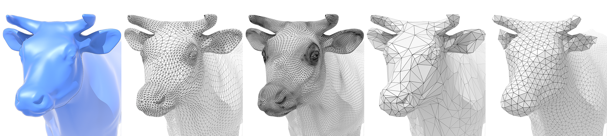
Subdivision (Upsampling)
Increase resolution
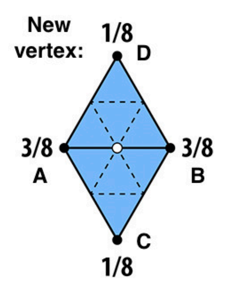
Loop Subdivision
Only for triangle faces
Intro more triangle meshes: Split triangles -> Update old / new vertices differently (according to weights)
- For new vertices: Update to
- For old vertices (e.g. degree 6 vertices): Update to

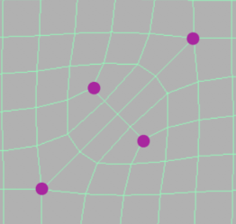
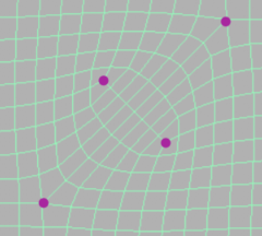
Catmull-Clack Subdivision (General Mesh)
Can be used for various types of faces
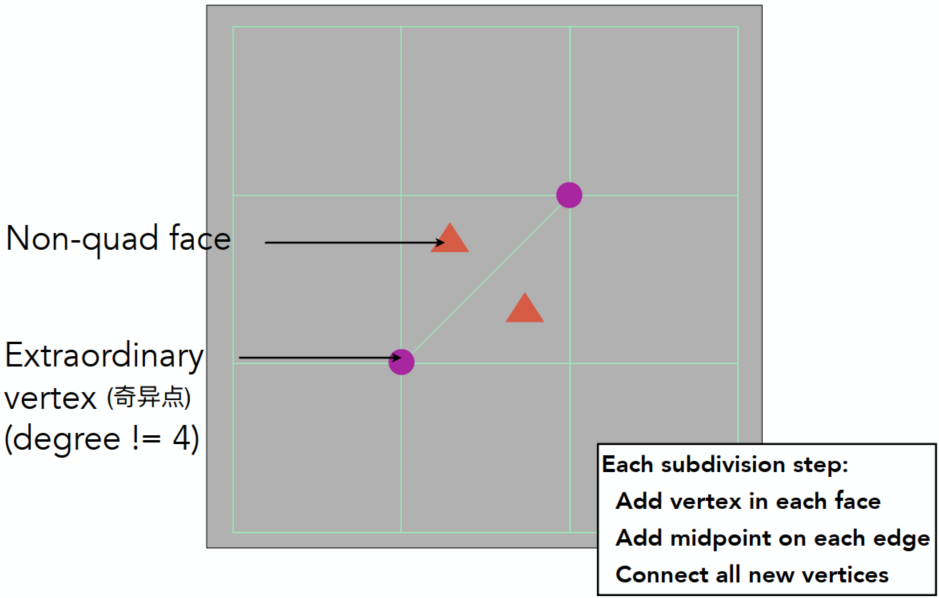
After several steps of Catmull-Clack subdivision:
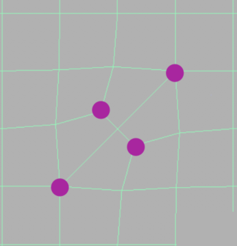
Vertex Updating Rules (Quad Mesh)

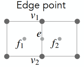
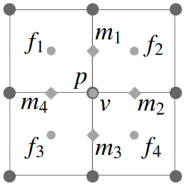
- Face Point:
- Edge Point:
- Vertex Point:
using the average to make it smoother => similar to the method of blur
Simplification (Downsampling)
Reduce the mesh amount to enhance performance
Edge Collapse
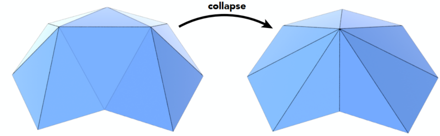
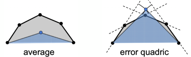
Quadric Error Metrics (geometric error introduced)
New vertex should minimize its sum of square distance (L2 distance) to previously related triangle planes
-> could cause error changes of other edges => dynamically update the other affected (prior queue / …)
=> Greedy algorithm for optimization (easy for flat, hard to curvature)
Regularization (Same #triangles)
Improve quality
Ray Tracing (Lec. 13-16)
Rasterization cannot handle global effects well (fast approximation with low quality, but real time). However, soft shadows / especially for light bounces more than once
Ray Tracing is usually off-line, accurate but very slow
Ray Tracing Basis
Light Rays
- Light travels in straight lines (not correct)
- Light rays do not “collide” with each other if they cross (still not correct)
- Light rays travel from the light sources to the eye (but the physics is invariant under path reversal - reciprocity)
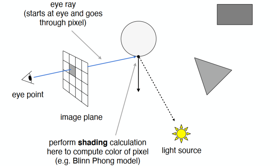
Ray Casting
Pinhole Camera Model
Generate an image by casting one ray per pixel
Check for shadows by sending a ray to the light
Generating Eye Rays
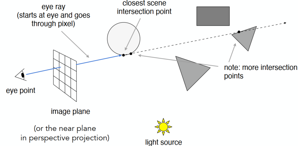
Shading Pixels (Local Only)
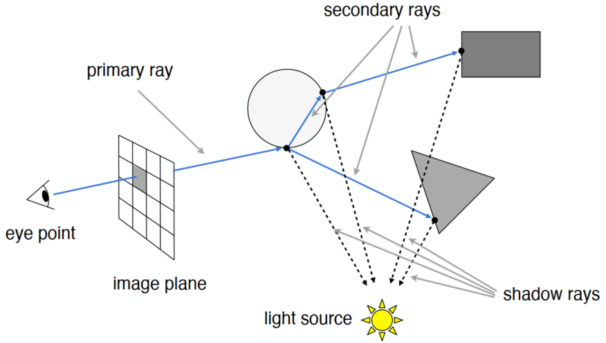
Recursive (Whitted-Style) Ray Tracing
Ray can travel through some (transparent / semi-transparent) media, but need to consider the energy loss
Ray-Surface Intersection
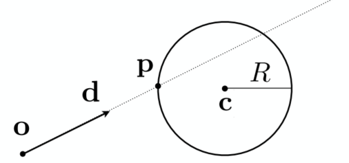
Ray Equation
Ray is defined by its origin and a direction vector
(
Ray Intersection
With Sphere
Sphere:
=> Solve for the intersection:
for a second order equation:
where
With Implicit Surface
- General implicit surface:
- Substitute ray equation:
Solve for real, positive roots:
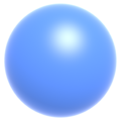

- Sphere:
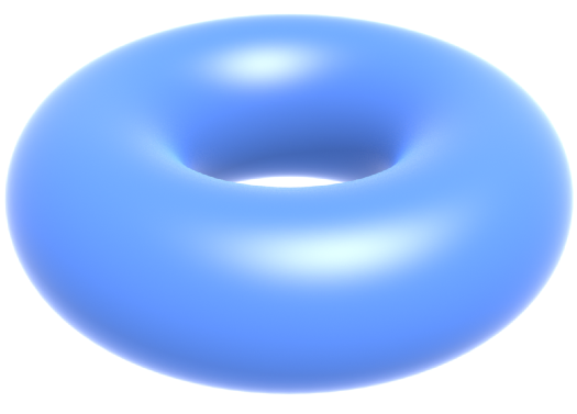
- Dohnut:
- 3D heart:
With Triangle Mesh
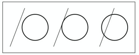
Idea: Just intersect ray with each triangle (too slow) => can have 0, 1 intersections (ignoring multiple intersections)
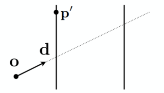
-> Triangle is a plane => Ray-plane intersection + Test if inside triangle
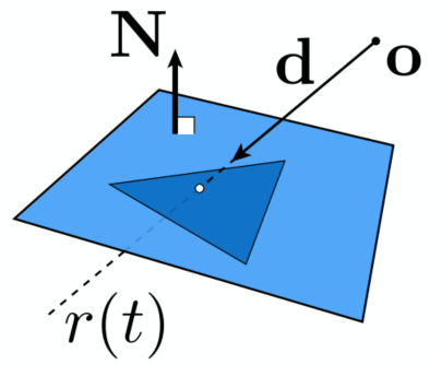
Plane Equation:
Solve for intersection:
Set
Möller Trumbore Algorithm (for triangle problem)
A faster approach, giving barycentric coordinate directly
RHS: represent any point in the plane (sum of the coefficients is 1)
Costs = 1 div, 27 mul, 17 add
Need to check if
Accelerating Ray-Surface (Triangle) Intersection
Problem: Naive algorithm (for every triangle) = #pixels x #triangles (x #bounces) (very slow)
Bounding Volumes
- Object fully contained in the volume
- If not hit the volume, it doesn’t hit the object
- Test BVol first then test object if it hits
Ray-AABB (Box) Intersection
Understanding: Box is the intersection of 3 pairs of slabs
Specifically: Axis-Aligned Bounding Box (AABB)
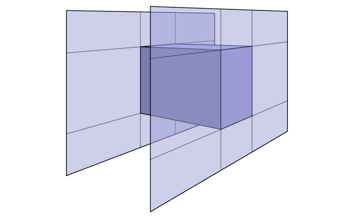
2D example: Compute intersections with slabs and take intersection of
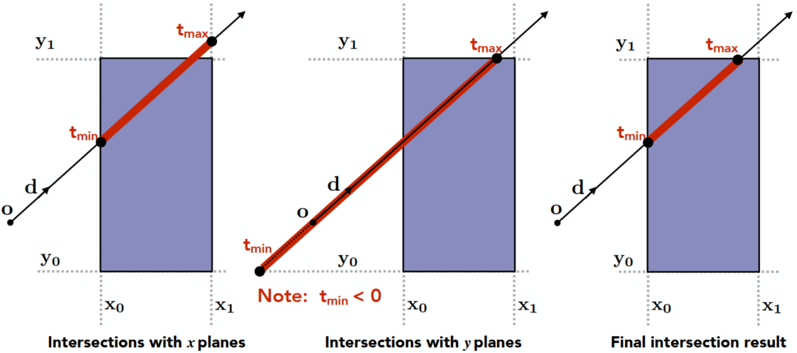
Key ideas:
- The ray enters the box only when it enters all pairs of slabs
- The ray exits the box as long as it exits any pair of slabs
For each pair, calculate the
For the 3D box:
Results:
If
But ray is not a line (should check whether
If
If
Summary: ray and AABB intersect iff:
Why Axis-Aligned:
Slab perpendicular to x-axis:
Acceleration with AABBs
Uniform Spatial Partitions (Grids)
Uniform Grids
Preprocess - Build Acceleration Grid
- Find bounding box
- Create grid
- Store each object in overlaping cells
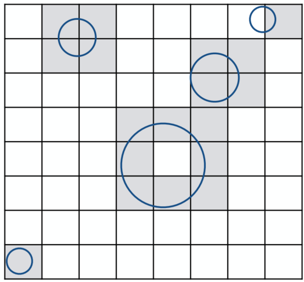
Ray-Scene Intersection
Find the first intersection (with the object) first. If found that the ray passes through a box in which there’s an obj -> test if intersects with the obj (NOT necessary)
(Ray intersect with boxes - fast; with obj - slower)
Step through grid in ray traversal order (-> similar to the method of drawing a line in the rasterization pipeline)

For each cell: test intersection with all objects stored at that cell
Resolution
Acceleration effects: One cell - no speedup; Too many cells - Inefficiency due to extraneous grid traversal
Heuristic: #cell = C * #objs; where C ≈ 27 in 3D
Usage
- Work well on large collections of objects that are distributed evenly in size and space
- Fail in “Teapot in a stadium” problem (distributed not evenly, a lot of empty space)
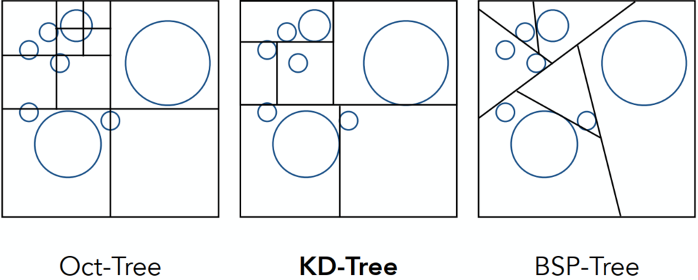
Spatial Partitions
Discretize the Bounding Boxes (in 3D)
Oct-Tree: Split the bounding boxes evenly (in 3D so 8 branches)
Stopping criteria -> until empty boxes / sufficiently small
KD-Tree: Always split the bounding box in different direction after another (horizontally or vertically, e.g., Horizontally first, then vertically, then horizontally again …; In 3D: x -> y -> z -> x -> …) => distribution almost evenly (Similar properties as binary-tree)
BSP-Tree: Not suitable for higher orders
KD-Tree
KD-Tree Pre-processing
Actually in every branch, the split should be applied every time (in the following plot, only show one of the splitted branch)
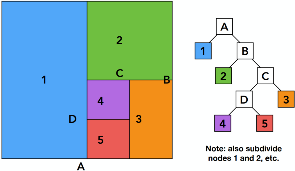
Data Structure for KD-Trees
Internal nodes store:
- Split axis: x-, y-, z-axis
- Split position: coordinate of split plane along axis
- Children: pointers to child nodes
- No obj are stored in internal nodes
Leaf nodes store:
- List of objs
Traversing a KD-Tree
For the outer box have intersection (internal node) -> consider the sub-nodes (split1)

In sub-nodes: Leaf 1 (LHS) & internal (RHS) both have intersections -> internal node splits -> … -> intersections found (after traversing all nodes)
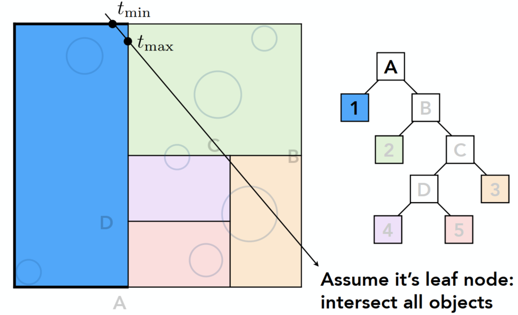
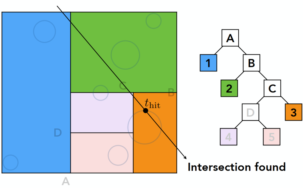
When have intersection with a leaf node of the box, the ray should find intersection with all the objects in this node
Problem:
- In 3D, KD-Tree is complex and not easy to be written (especially when triangles intersects with the box but not inside the box, …)
- Some objects can be counted several times (appears in various of leaf nodes)
Object Partitioning & Bounding Volume Hierarchy (BVH)
According to objects other than space, very popular
Main Idea
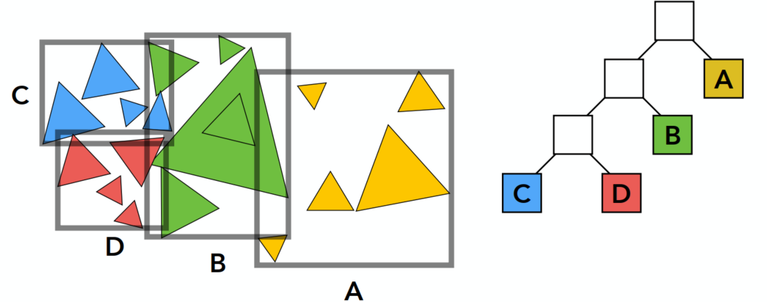
Can introduce some spec. stopping criteria
Property: No triangle-box intersections / No obj appears in more than one boxes
Problem: Boxes can overlap -> more researches to split obj
Summary: Building BVHs
- Find bounding box
- Recursively split set of objects in 2 subsets
- Recompute the bounding box of the subsets
- Stop when necessary
- Store objects in each leaf nodes
Subdivide a node:
- Choose a dimension to split
- Heuristic #1: Always choose the longest axis in node
- Heuristic #2: Split node at location of median objects (amount balance) -> quick splitting
Termination criteria:
- Heuristic: node contains few elements (e.g, < 5)
BVH Traversal (Pseudo Code)
xxxxxxxxxxIntersect(Ray ray, BVH node) { if (ray misses node.bbox) return; if (node is leaf node) test intersection with all objs; return closest intersection; hit1 = Intersect(ray, node.child1); hit2 = Intersect(ray, node.child2); // recursive return the closer of hit1, hit2;}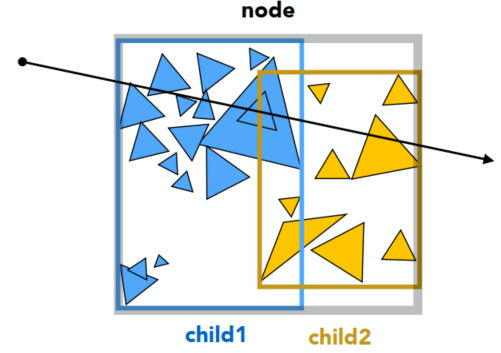
Radiometry
Measurement system and units for illumination
Accurately measure the spatial properties of light
Terms: Radiant flux(辐射通量), intensity, irradiance(辐射照度), radiance(辐射亮度)
-> Light emitted from a source (radiant intensity) / light falling on a surface (irradiance) / light traveling along a ray (radiance)
Perform lighting calculations in a physically correct manner
Radiant Energy and Flux (Power)
Radiant energy is the energy of electromagnetic radiation. Measured in units of joules:
Radiant flux (power) is the energy emitted, reflected, transmitted or received per unit time:
Flux - #photons flowing through a sensor in unit time
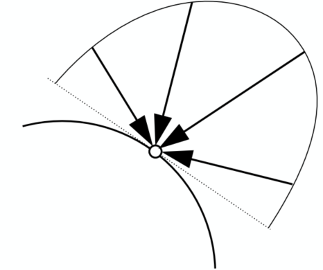
Radiant Intensity
The radient (luminous) intensity is the power per unit solid angle(立体角) emitted by a point light source (candela is one of the SI units) (sr - solid radius)
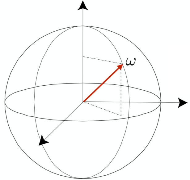
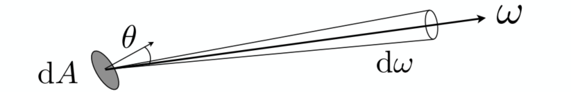
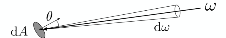
Angles and Solid Angles
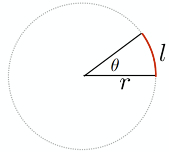
- Angle: ratio of subtended arc length on circle to radius
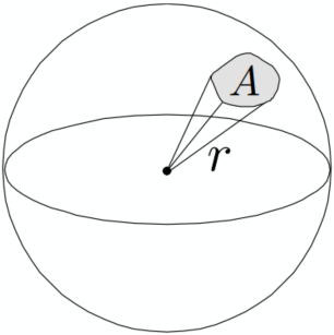
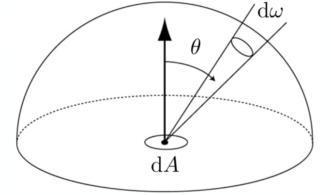
- Solid Angle: ratio of subtended area on sphere to radius squared
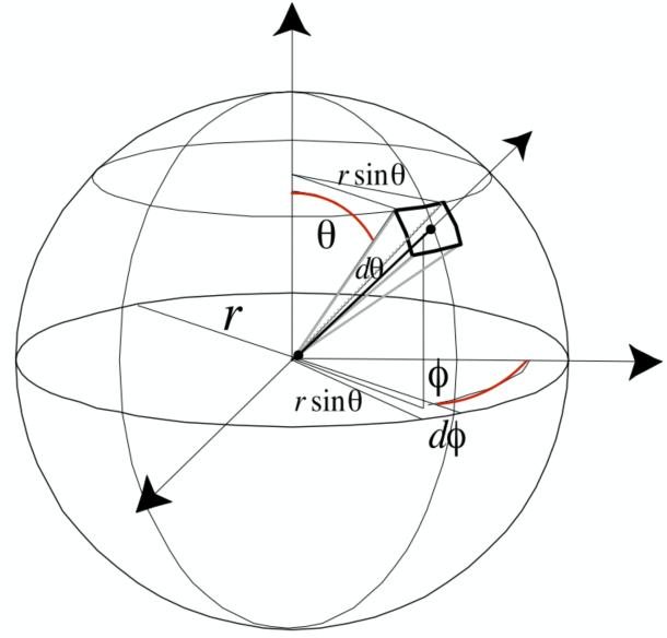
Differential Solid Angles: (The unit area of the differential retangular)
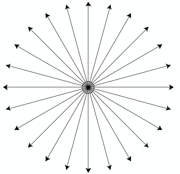
Isotropic Point Source
Irradiance
The irradiance is the power per (perpendicular/projected) unit area incident on a surface point
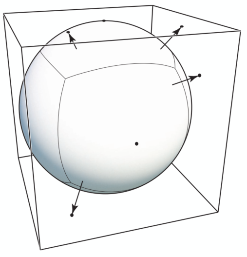
Lambert’s Cosine Law
-> Remind Blinn-Phong model / Seasons occur
Irradiance at surface is proportional to cosine of angle between light dir and surface normal
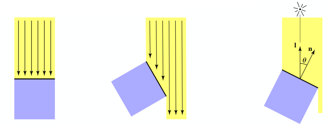
- Top face of cube receives a certain amount of power:
- Top face of 60% rotated cube receives half power:
- In general, power per unit area is proportional to
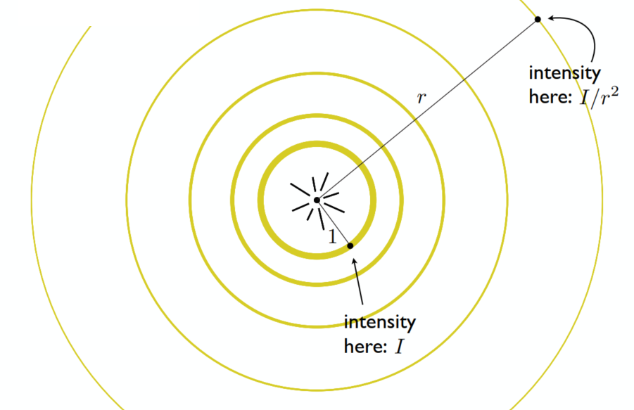
Irradiance Falloff
Recall -> Blinn-Phong’s Model
Assume light is emitting power
- distance = 1:
- distance = r:
Radiance
Radiance is the fundamental field quantity that describes the distribution of light in an environment
- Quantity associated with a ray
- All about computing radiance
The radiance (luminance) is the power emitted, reflected, transmitted or received by a surface, per unit solid angle, per projected unit area (two derivatives) -> the
-> Recall:
- Irradiance: power per projected unit area
- Intensity: power per solid angle
Then: Radiance: Irradiance per solid angle / Intensity per projected unit area
Incident Radiance
Incident radiance is the irradiance per unit solid angle arriving at the surface
=> it is the light arriving at the surface along a given ray (point on surface and incident direction)
Exiting Radiance
Exiting surface radiance is the intensity per unit projected area leaving the surface
e.g., for an area light it is the light emitted along a given ray (point on surface and exit direction).
Irradiance vs. Radiance
- Irradiance: total power received by area
- Radiance: power received by area
(
Bidirectional Reflectance Distribution Function (BRDF)
The function to indicate the property of reflection (smooth surface / rough surface)
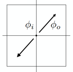
Reflection at a Point
Radiance from direction
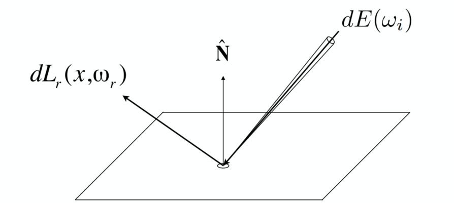
- Differential irradiance incoming:
- Differential radiance exiting (due to
BRDF
The BRDF represents how much light is reflected into each outgoing dir
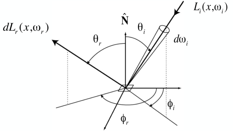
BRDF defines the material
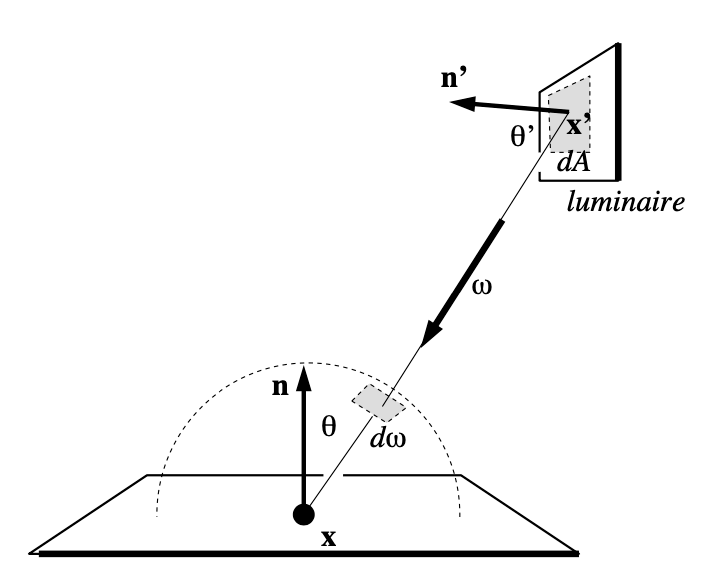
The Reflection Equation
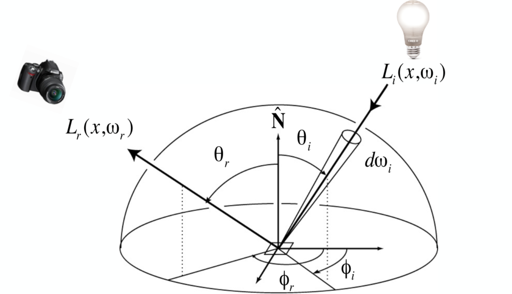
Challenge: Recursive Equation
Reflected radiance depends on incoming radiance; but incoming radiance depends on reflected radiance (at another point in the scene) <- the lights will not just bounce once
The Rendering Equation
For objects can emit light -> adding an emission term to make the reflection function general (
Note: now assume that all dir are pointing outwards
Understanding the Rendering Equation
Yellow - Large light source; Blue - Surfaces (interreflection)
is a Fredholm Integral Equation of second kind [extensively studied numerically] with canonical form
The kernel of equation replaced with the Light Transport Operator
=> solve the rendering equation: discretized to a simple matrix equation [or system of simultaneous linear equations: L, E are vectors, K is the light transport matrix] => Applying binomial theorem
Global Illumination
In ray tracing => Global Illumination (Higher order K)
- E: Emission directly from light sources -> Shading in Rasterization
- KE: Direct illumination on surfaces -> Shading in Rasterization
- K2E: Indirect illumination (One bounce) [mirrors, refraction]
- K3E: Two bounce in direct illum.
- …
Monte Carlo Path Tracing
Probability Review
Random Variables
| Type | Description |
|---|---|
| Random variable, represents a distribution of potential values | |
| Probability density function (PDF), describing relative probability of a random process choosing value |
Uniform PDF: all values over a domain are equally likely
Probabilities
n discrete values
Requirements of a probability distribution:
Expected Value
Expected value of
Continuous Case: Probability Density Function
Conditions on
Expected value:
Function of a Random Value
=> Expected value:
Monte Carlo Integration
We want to solve an integral but it can be too hard to solve analytically => Monte Carlo (numerical method)
Definite integral
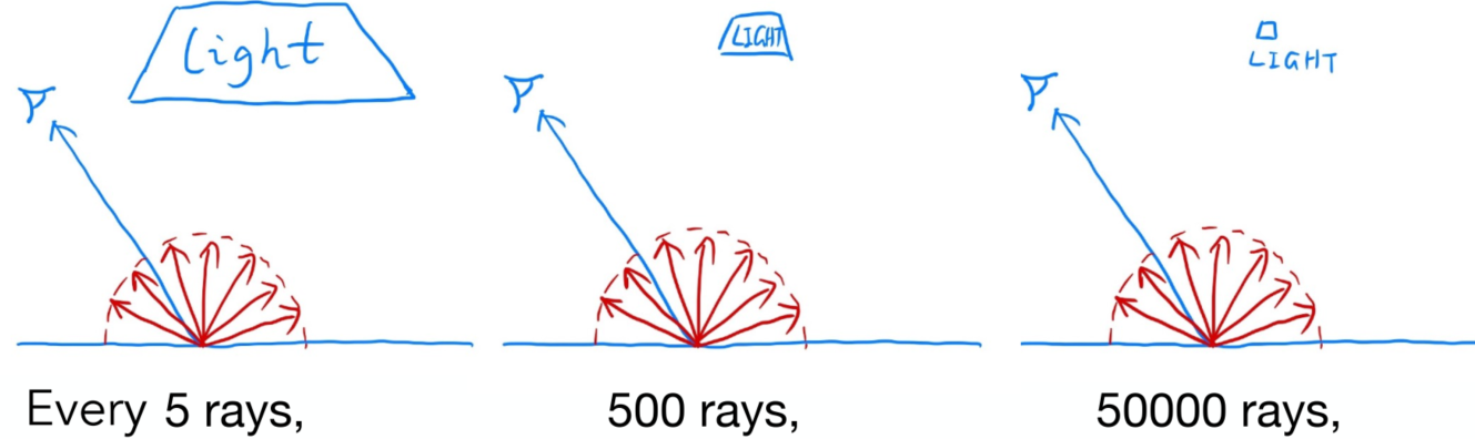
Monte Carlo estimator:
- The more samples, the less variance
- Sample on
Path Tracing
Motivation: Whitted-Style RT
Whitted-style ray tracing
- Always perform specular reflections / refractions
- Stop bouncing at diffuse surfaces
Problems => Not 100% reasonable
- The reflections can be divided into glossy (rough surface) and mirror (specular) => Witted-Style cannot present the glossy result
- Diffuse material can also reflect light (but to many directions), resulting in color bleeding (global illumination can present) -> Witted-Style doesn’t bounce light on diffuse surface (= direct illumination)
The Whitted-Style is not that correct -> But the rendering equation is correct
But involves: solving an integral over the hemisphere (=> Monte Carlo) and recursive execution
A Simple Monte Carlo Solution
Suppose we want to render one pixel (point) in the following scene for direct illumination only
For the reflection equation:
Consider the direction as the random variable, want to compute the radiance at
Monte Carlo integration:
and pdf:
=> In general:
Algorithm: (Direct illumination)
xxxxxxxxxxshade(p, wo) Randomly choose N directions wi~pdf Lo = 0.0 For each wi Trace a ray r(p, wi) If ray r hit the light Lo += (1 / N) * L_i * f_r * cosine / pdf(wi) Return LoIntroducing Global Illumination
Further step: what if a ray hits an object?
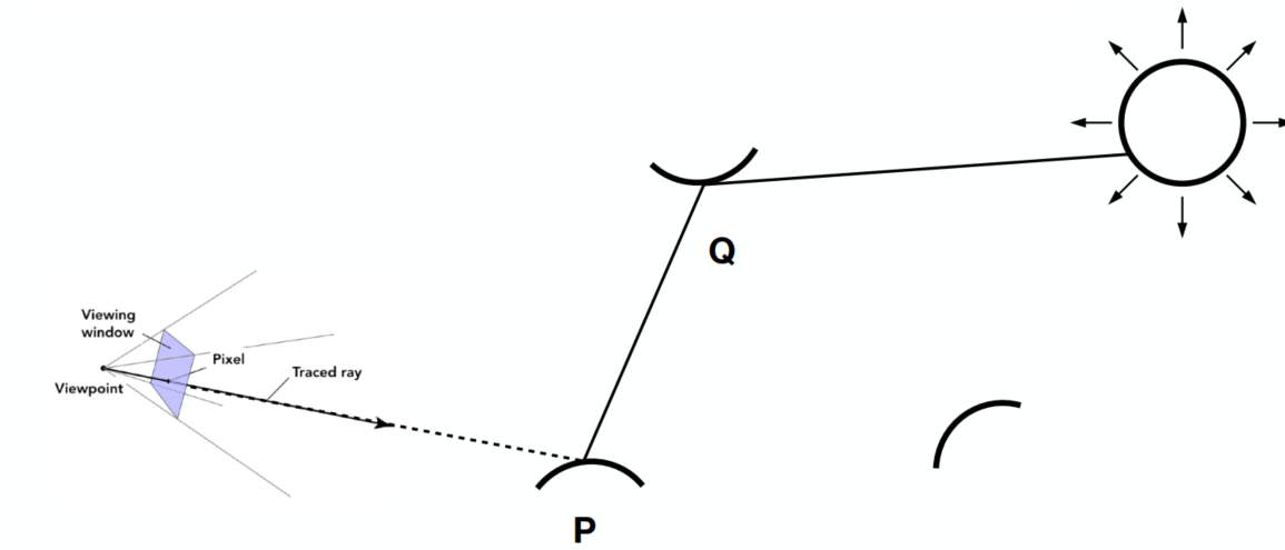
Q also refects light to P => = the dir illum at Q
New Algorithm:
xxxxxxxxxxshade(p, wo)Randomly choose N directions wi~pdfLo = 0.0For each wiTrace a ray r(p, wi)If ray r hit the lightLo += (1 / N) * L_i * f_r * cosine / pdf(wi)Else If ray r hit a object at qLo += (1 / N) * shade(q, -wi) * f_r * cosine / pdf(wi) // new step!Return Lo
Problems:
Explosion of #rays as #bounces go up: #rays = N#bounces (#rays will not explode iff N = 1)
From now on => always assume that only 1 ray is traced at each shading point => Actual Path Tracing (Shown in Path Tracing Algorithm)
=> Noisy if N = 1: Tracing more paths through each pixel and average the radiance (Shown in Ray Generation)
Recursive in
shade(): never stopbut the light does not stop bouncing indeed / cutting #bounce == cutting energy
=> Russian Roulette (RR), shown below
Path Tracing Algorithm: (Recursive)
xxxxxxxxxxshade(p, wo)Randomly choose ONE direction wi~pdf(w)Trace a ray r(p, wi)If ray r hit the lightReturn L_i * f_r * cosine / pdf(wi)Else If ray r hit an object at qReturn shade(q, -wi) * f_r * cosine / pdf(wi)
Ray Generation
Tracing more paths through each pixel and average the radiance (similar to ray casting in ray tracing)
xxxxxxxxxxray_generation(camPos, pixel)Uniformly choose N sample positions within the pixelpixel_radiance = 0.0For each sample in the pixelShoot a ray r(camPos, cam_to_sample)If ray r hit the scene at ppixel_radiance += 1 / N * shade(p, sample_to_cam)Return pixel_radiance
Rusian Roulette (RR)
Basic Idea:
- With probability 0 < P < 1, you are fine
- With probability 1 - P, otherwise
Previously, always shoot a ray at a shading point and get the result Lo
Suppose we can manually set a probability P (0 < P < 1):
- With P, shoot a ray and return the shading result divided by P (Lo/P)
- With 1-P, don’t shoot a ray and get 0
=> the expected value is still Lo:
Algorithm with RR: (real correct version)
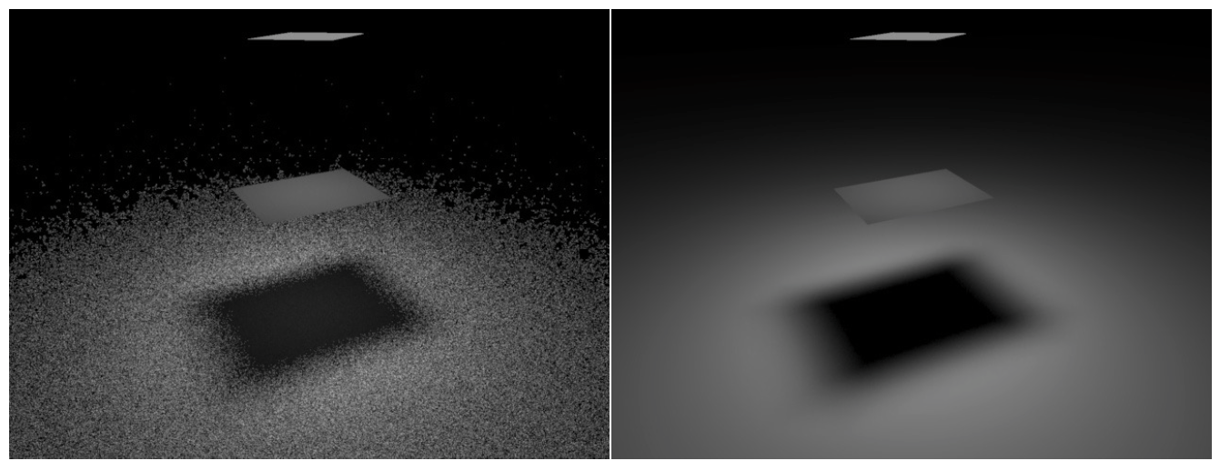
xxxxxxxxxxshade (p, wo)    Manually specify a probability P_RR    Randomly select ksi in a uniform dist. in [0, 1]    If (ksi > P_RR) return 0.0;
    Randomly choose ONE direction wi~pdf(w)    Trace a ray r(p, wi)    If ray r hit the light        Return L_i * f_r * cosine / pdf(wi) / P_RR    Else If ray r hit an object at q        Return shade(q, -wi) * f_r * cosine / pdf(wi) / P_RR
Samples Per Pixel (SPP) => low (left): noisy
Problem:
- Not efficient
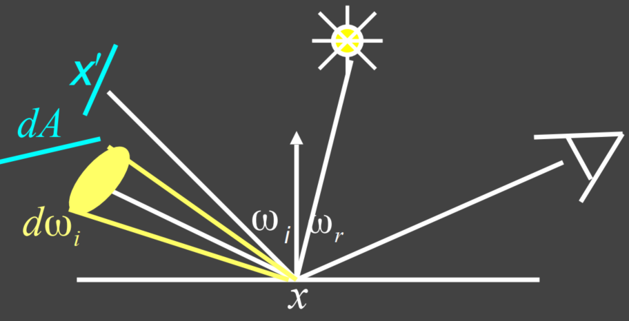
Sampling the Light
For area light sources, the ones with bigger areas have higher probability to get hit by the the “ray” if uniformly sample the hemisphere at the shading point => waste
Monte Carlo method allows any sampling method => make the waste less
Assume uniformly sampling on the light:
But the rendering equation integrates on the solid angle:
Projected area on the unit sphere:
Rewrite the rendering equation with
Now integrate on the light =>
Now we consider the radiance coming from 2 parts:
- Light source (direct, no need for RR)
- Other reflections (indirect, RR)
Light Sampling Algorithm:
xxxxxxxxxxshade(p, wo) # Contribution from the light source. (no RR) Uniformly sample the light at x’ (pdf_light = 1 / A) L_dir = L_i * f_r * cos θ * cos θ’ / |x’ - p|^2 / pdf_light # Contribution from other reflectors. (with RR) L_indir = 0.0 Test Russian Roulette with probability P_RR Uniformly sample the hemisphere toward wi (pdf_hemi = 1 / 2pi) Trace a ray r(p, wi) If ray r hit a non-emitting object at q L_indir = shade(q, -wi) * f_r * cos θ / pdf_hemi / P_RR Return L_dir + L_indirFinal: how to know if the sample on the light is not block or not?
xxxxxxxxxx# Contribution from the light source.L_dir = 0.0Uniformly sample the light at x’ (pdf_light = 1 / A)Shoot a ray from p to x’If the ray is not blocked in the middle L_dir = …
Materials and Appearances (Lec. 17)
Material == BRDF
Materials
Diffuse / Lambertian Material
Light is equally reflected in each output dir (
Suppose the incident light is uniform (identical radiance). According to energy balace, incident and exiting radiance are the same.
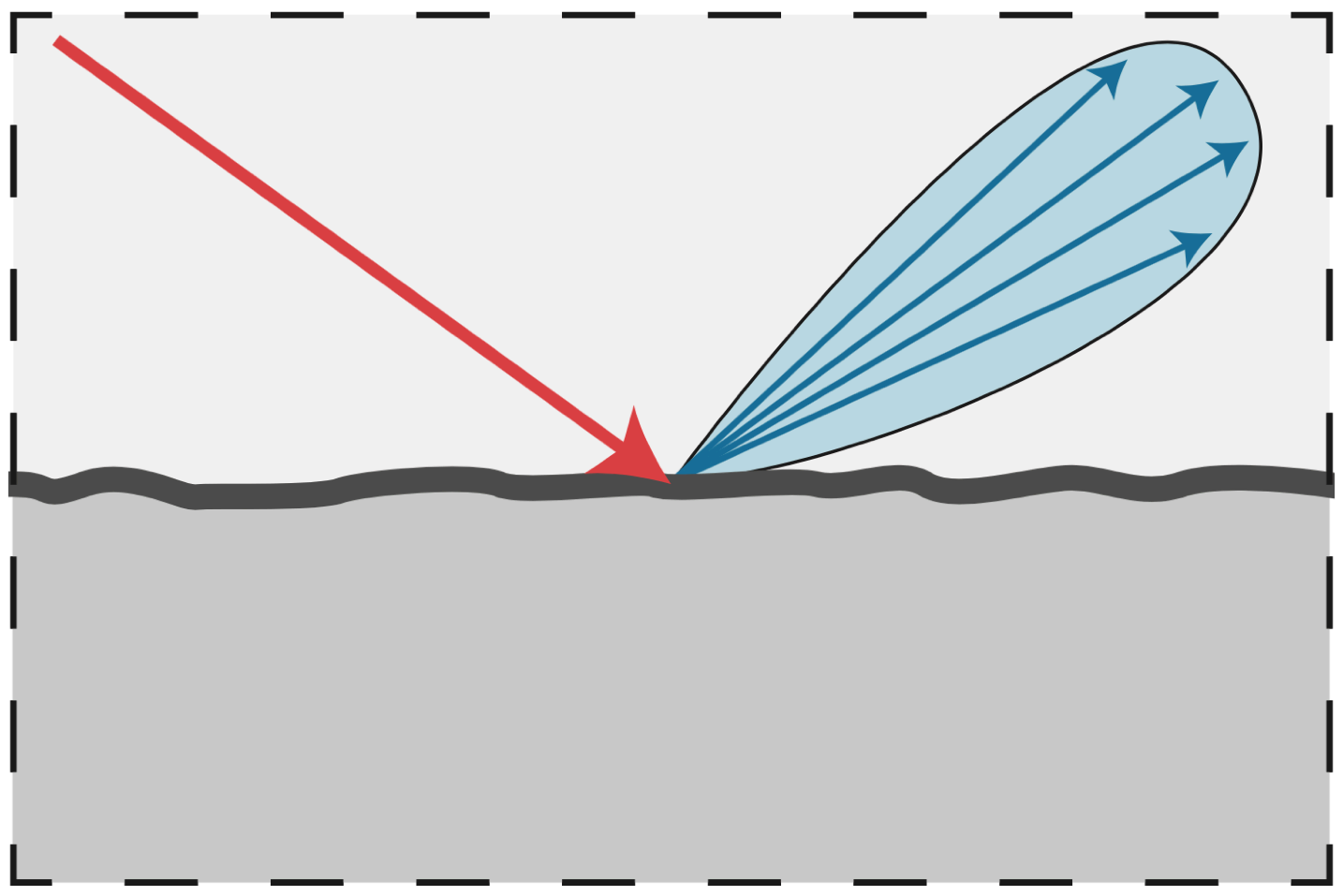
Glossy Material (BRDF)
Air <-> copper / aluminum
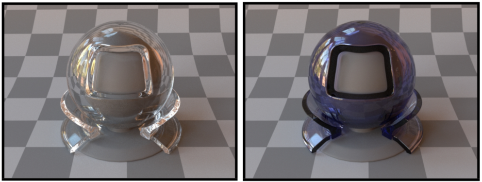
Ideal Reflective / Refractive Material (BSDF*)
Air <-> water interface / glass interface (with partial abs)
-> the “S” in “BSDF” is for “Scatter” => both reflection and refraction are ok
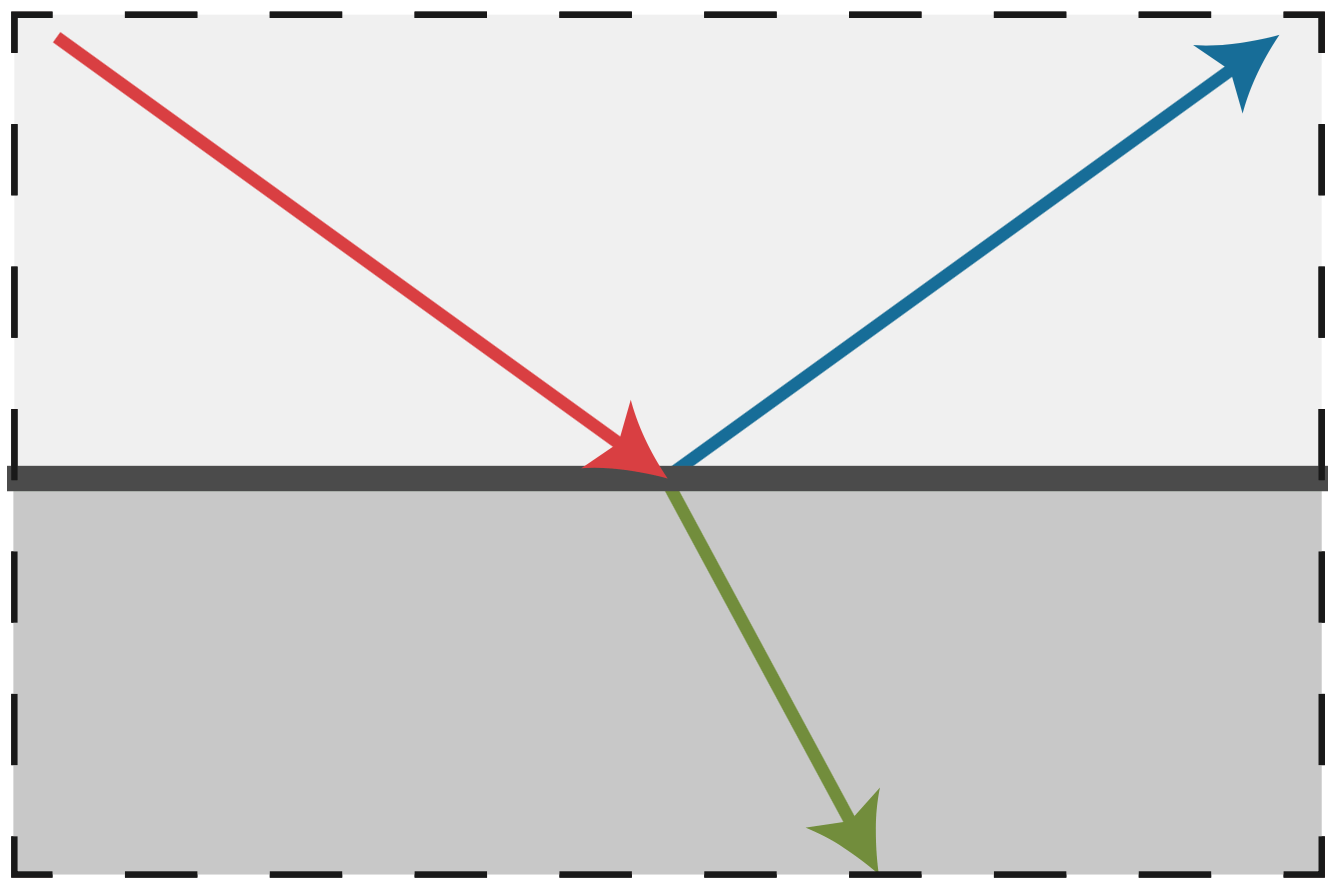
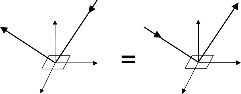
Reflection & Refraction
Perfect Specular Reflection
Left:
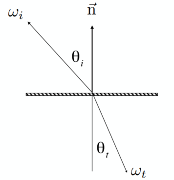
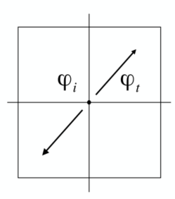
Specular Refraction
Light refracts when it enters a new medium
Snell’s Law
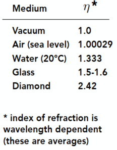
Transmitted angle depends on: Index of refraction (IOR) for incident and exiting ray
Left:
*Diamond has a very high refraction rate, which means that the light will be refracted heavily inside the diamonds => shiny with various colors
Want a reasonable real number to have the refraction occurred (need
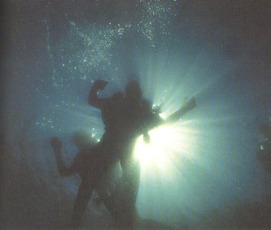
Total internal reflection: The internal media has a higher refraction rate than outside:
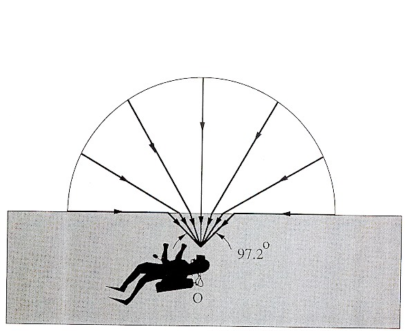
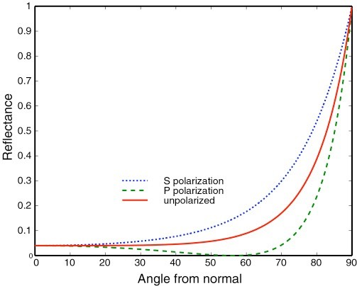
Fresnel Reflection / Term
Reflectance depends on incident angle (and polarization of light)
e.g., reflectance increases with grazing angle
Dielectric (
Conductor
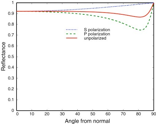
Formulae:
Accurate: (considering the polarization)
Approximation: Schlick’s approximation
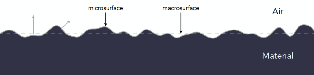
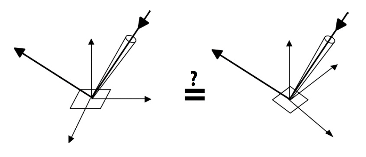
Microfacet Material
Microfacet Theory
View from far away: material and appearance; from nearby: geometry
Rough Suface:
- Macroscale: flat & rough
- Microscal: bumpy & specular
Individual elements of surface act like mirrors
- Known as Microfacets
- Each microfacet has its own normal
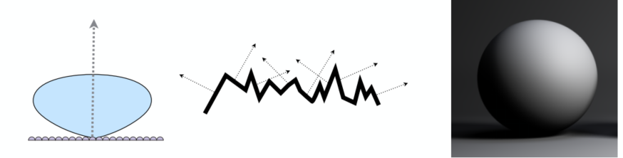
Microfacet BRDF
Key: the distribution of microfacets’ normals => the roughness
concentrated distributed <==> glossy
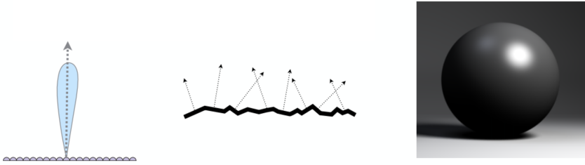
spread distributed <==> diffuse
Microfacets are mirrors
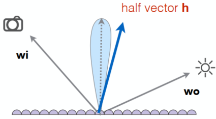
(
Isotropic / Anisotropic Materials (BRDFs)
Key: directionality of underlying surface (following are the surface normals and the BRDF with fixed wi and varied wo)
Isotropic: if different oriented azimuthal angles of incident and reflected rays give the same BRDFs, the material is isotropic
Anisotropic (strongly directional)

Reflection depends on azimuthal angle
Results from oriented microstructure of surface, e.g., brushed metal, nylon, velvet
Properties of BRDFs
Non-negativity:
Linearity:
Reciprocity principle:
Energy conservation: (the convergence of path tracing)
Isotropic vs. anisotropic
- If isotropic:
- from reciprocity:
- If isotropic:
Measuring BRDFs
Image-Based BRDF Measurement
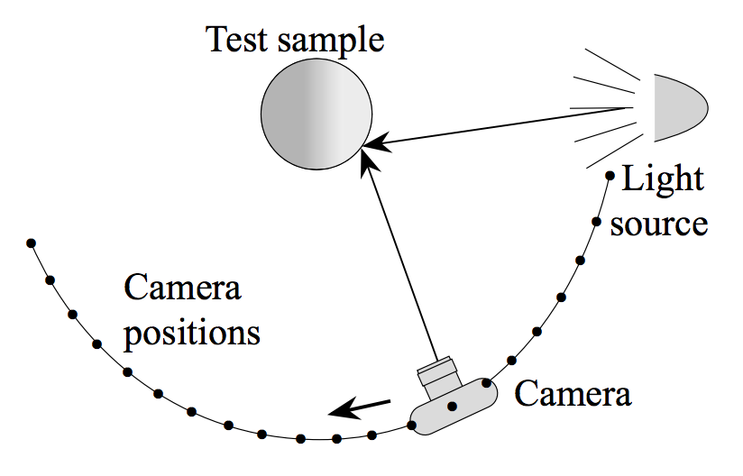
Instrument: gonioreflectometer
General approach: (curse of dimensionality)
for each outgoing dir wo move light to illuminate surface with a thin beam from wo for each incoming dir wi move sensor to be at dir wi from surface measure the incident radiance
Improving efficiency:
- Isotropic surfaces reduce dim from 4d -> 3d
- Reciprocity reduce # of measurements by half
- Clever optical systems
…
-> Important lib for BRDFs: MERL BRDF Database
Advanced Topics in Rendering (Lec. 18)
Advanced light transport and materials
Advaced Light Transport
Unbiased light transport methods
- Bidirectional path tracing (BDPT)
- Metropolis light transport (MLT)
Biased light transport methods
- Photon mapping
- Vertex connection and merging (VCM)
Instant radiosity (VPL / many light methods)
Biased vs. Unbiased Monte Carlo Estimators
- An unbiased Monte Carlo doesn’t have any systematic error (No matter how many samples -> always expect the correct result)
- Otherwise, biased (special case: expected value converges to the correct value as infinite #samples are used #samples are used - consistent)
Unbiased Light Transport Methods
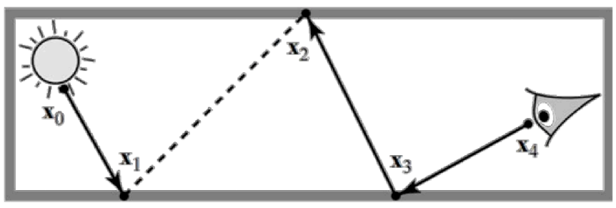
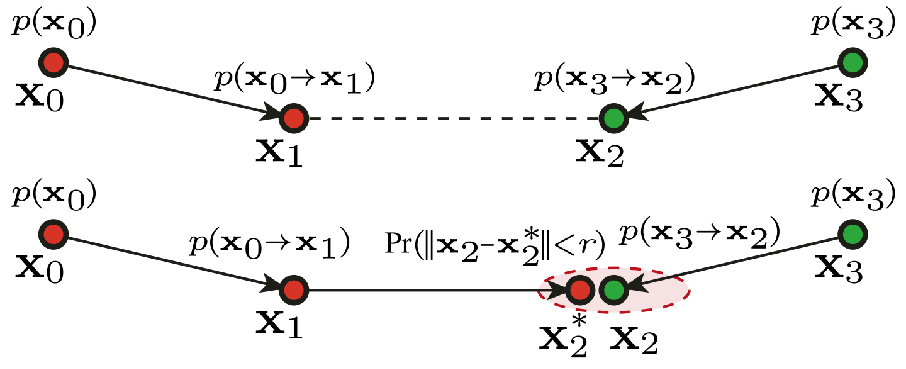
Bidirectional Path Tracing (BDPT)
A path connects the camera and the light
BDPT: Traces sub-paths from both the cam and the light; connects the end pts from both sub-paths
Properties:
- Suitable if the light transport is complex on the light’s side
- Difficult to implement & quite slow
Metropolis Light Transport (MLT)
A Markov Chain Monte Carlo (MCMC) application
Jumping from the current samplke to the next with some PDF
Key idea: Locally perturb an existing path to get a new path
Good at locally exploring difficult light paths
Properties:
- Works great with difficult light paths
- Difficult to estimate the convergence rate; doesn’t guarantee equal convergence rate per pixel; usually produces “dirty” results => Usually not used to render animations
Biased Light Transport Methods
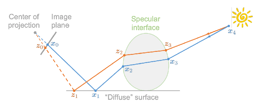
Photon Mapping
A biased approach & A two-stage method -> Good at handling Specular-Diffuse-Specular (SDS) paths and generating caustics
Approach (variations apply):
Stage 1 - Photon tracing: Emitting photons from the light source, bouncing them around, then recording photons on diffuse surfaces
Stage 2 - Photon collection (final gathering): Shoot sub-paths from the camera, bouncing them around, until they hit diffuse surfaces
Calculation: Local density estimation
Areas with more photons should be brighter. For each shading point find the nearest N photon. Take the surface area they over. (Density = Num / Area)
Smaller
Biased method problem: local density est:
=> Bisaed == blurry; Consistent == not blurry with inf #samples
Vertex Connection and Merging (VCM)
A Combination of BDPT and Photon Mapping
Key: Not waste the sub-paths in BDPT if their end pt cannot be connected but can be merged; use photon mapping to handle the mergeing of nearby photons
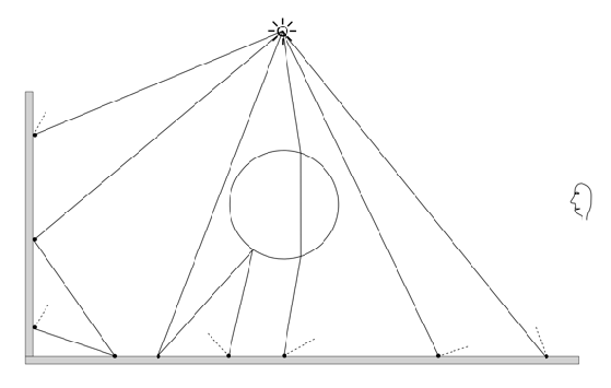
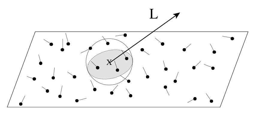
Instant Radiosity (IR)
= Many-light approaches
Key: Lit surfaces can be treated as light sources
Approach:
- Shoot light sub-paths and assume the end point of each sub-path is a Virtual Point Light (VPL)
- Render the scene as usual using these VPLs
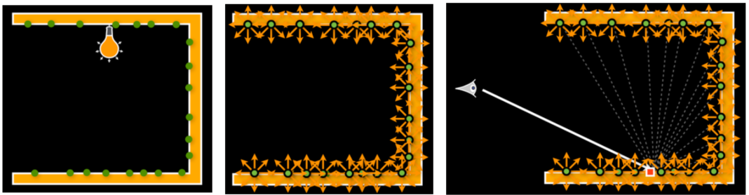
Properties:
- Fast and usually gives good results on diffuse scenes
- Spikes will emerge when VPLs are close to shading points; Cannot handle glossy materials
Advanced Appearance Modeling
Non-surface models => many stuff seems like surface model but actually non-surface
- Participating media
- Hair / fur / fiber (BCSDF)
- Granular material
Surface models
- Translucent material (BSSRDF)
- Cloth
- Detailed material (non-statistical BRDF)
Procedural appearance
Non-Surface Models
Participating Media
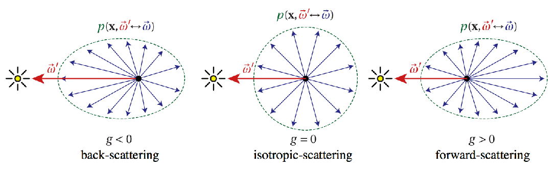
At any point as light travels through a participating medium, it can be (partially) absorbed and scattered (cloud / …)
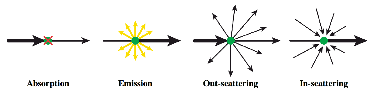
Use Phase Function (how to scatter) to describe the angular distribution of light scattering at any point
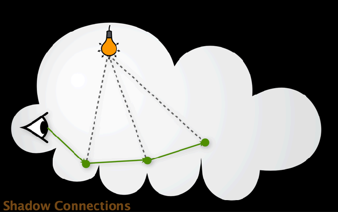
Rendering:
- Randomly choose a direction to bounce
- Randomly choose a distance to go straight
- At each ‘shading point’, connect to the light
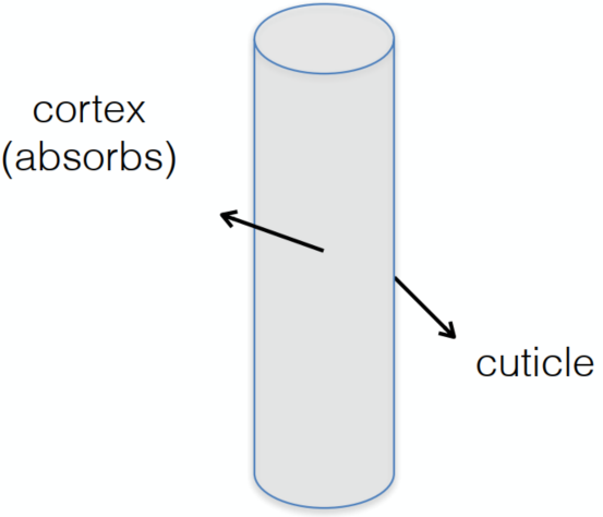
Hair Appearance
Light not on a surface but on a thin cylinder (Hightlight has 2 types: color and colorless)
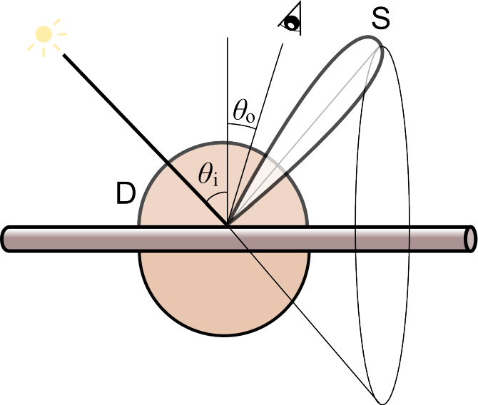
Kajiya-Kay Model
diffuse + scatter (form a cone zone) => not real
Marschner Model
(widely used model) => very good results
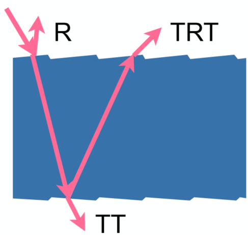
some reflected R and some penantrated (refraction) T (-> TT / TRT /…)
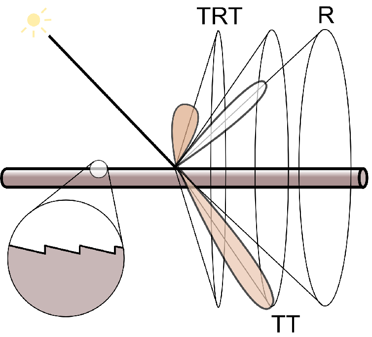
Glass-like cylinder (black -> absorb more; brown / bronde -> absorb less => color) + 3 types of light interactions (R / TT / TRT)
=> extremely high costs
Fur Appearance
cannot just simply apply human hairs => different in biological structures
Common: 3 layer structure

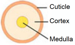
Difference: fur in animal has much bigger medulla (髓质) than human hair => more complex refraction inside (Need to simulate medulla for animal fur)
Double Cylinder Model
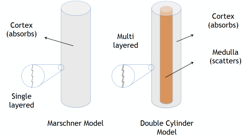
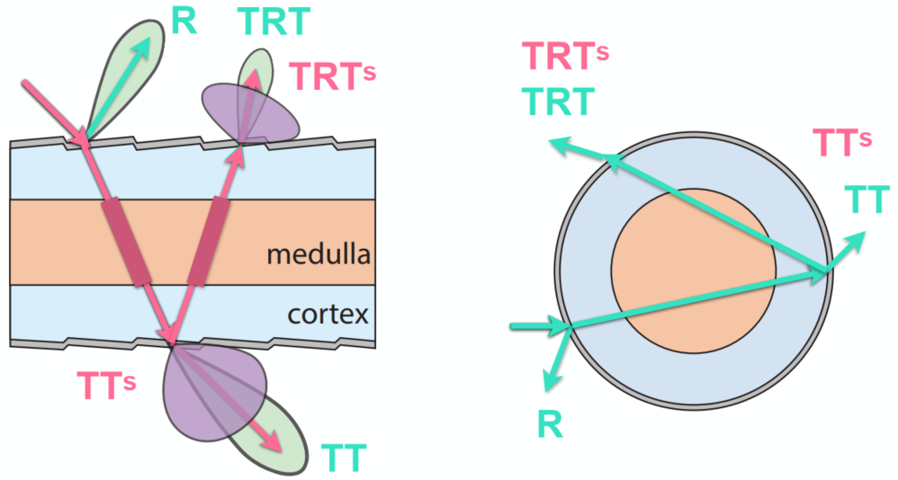
Add 2 scattered model => TTs and TRTs
Granular Material
avoid explicit modeling => procedural definition
Surface Models
Translucent Materials
Jellyfish / Jade / …
Subsurface Scattering
light exiting at different points than it enters
Actually violates a fundamental assumption of the BRDF (on the diffuse surface with BRDF, light reflects at the same point)
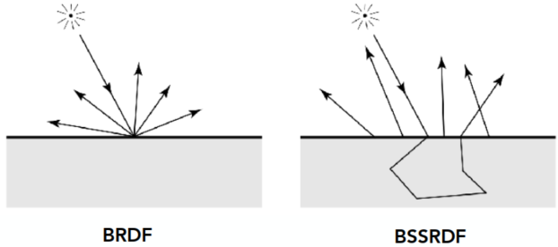
Scattering functions:
BSSRDF: generalization of BRDF; exitant radiance at one point due to incident differential irradiance at another point:
=> integrating over all points on the surface (area) and all directions
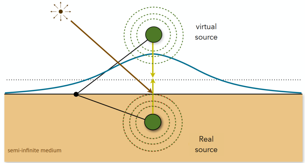
Dipole Approximation
Approximate light diffusion by introducing two point sources
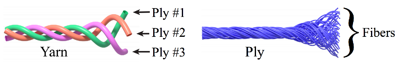
Cloth
A collection of twisted fibers (different levels of twist: fibers -> ply -> yarn)
Render as Surface
Given the weaving pattern, calculate the overall behavior (using BRDF)
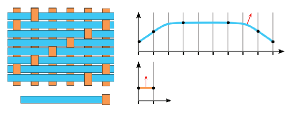
=> limitation: anisotropic cloth
Render as Participating Media
Properties of individual fibers & their distribution -> scattering parameters
=> Really high costs
Render as Actual Fibers
Render every fiber explicitly
=> Similar to hair, extremely high costs
Detailed Appearance
The now renderers are not good => too perfect results (reality: straches / pores / …)
Recap: Microfacet BRDF
Surface = Specular microfacets + Statistical normals
(
Define Details: required very high resolution normal maps
=> too difficult for rendering: for bumpy specular surface -> hard to catch from both cam or light source
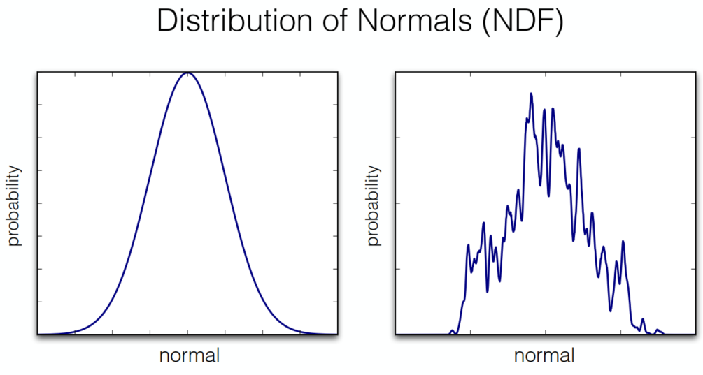
Solution: BRDF over a pixel
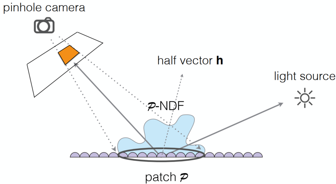
p-NDFs have sharp features
=> ocean waves / scratch / …
Recent Trend: Wave optics (for too micro / short time duration) other than geometric optics
Procedural Appearance
define details without textures => compute a noise function on the fly
- 3D noise -> internal structure
- hresholding (noise -> binary noise)
Cameras, Lenses and Lightings (Lec. 19)
Imaging = Synthesis + Capture
The sensor records the irradiance
Field of View (FOV)
Effect of Focal Lenght on FOV
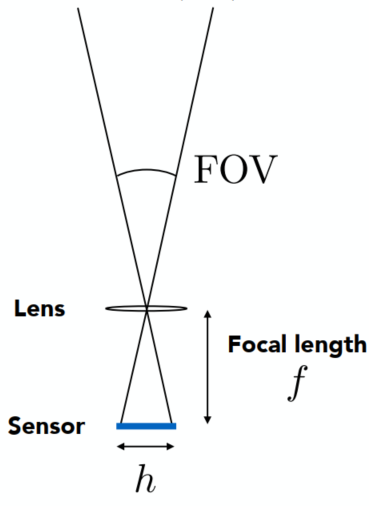
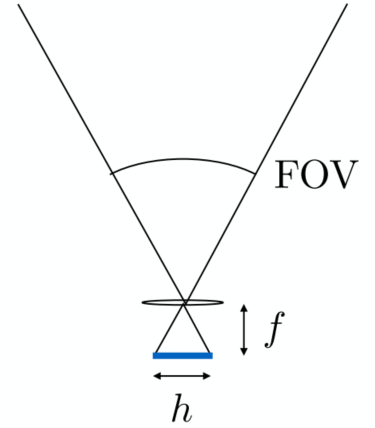
For a fixed sensor size, decreasing the focal length increases the field of view (assuming the sensor is fully used)
The referred focal lengh of a lens used on a 35mm-format film (36 x 24 mm)
-> e.g., 17 mm is wide angle 104°; 50 mm is a “normal” lens 47°; 200 mm is a telephoto lens 12°
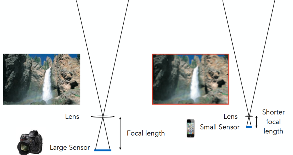
Effect of Sensor Size on FOV
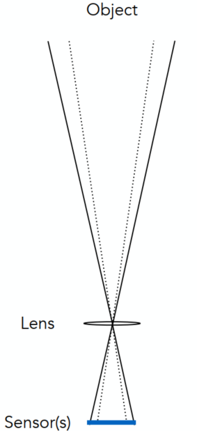
Maintain FOV on smaller sensor? => shorter focal length
Exposure
Exposure
- Time: controlled by shutter
- Irradiance: power of light falling on a unit area of sensor; controlled by lens aperture and focal lenth
Exposure Controls
Aperture size
Change the f-stop (Exposure levels) by opening / closing the aperture (iris control)
FNorF/N: the inverse-diameter of a round apertureThe f-number of a lens is defined as the focal length divided by the diameter of the aperture
Shutter speed (causes motion blur in slower speed / rolling shutter)
- Change the duration the sensor pixels integrate light
ISO gain (Trade sensitivity of grain / noise)
- Change the amplification (analog / digital) between the sensor values and digital image values
Some pairs
| F-stop | 1.4 | 2.0 | 2.8 | 4.0 | 5.6 | 8.0 | 11.0 | 16.0 | 22.0 | 32.0 |
|---|---|---|---|---|---|---|---|---|---|---|
| Shutter | 1/500 | 1/250 | 1/125 | 1/60 | 1/30 | 1/15 | 1/8 | 1/4 | 1/2 | 1 |
Fast and Slow Photography
High-Speed Photography
Normal exposure = extremely fast shutter speed x (large aperture and/or high ISO)
Long-Exposure Photography
Thin Lens Approximation
Real Lens Elements Are Not Ideal – Aberrations
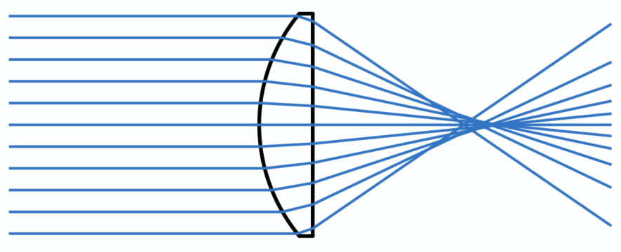
Ideal Thin Lens – Focal Point
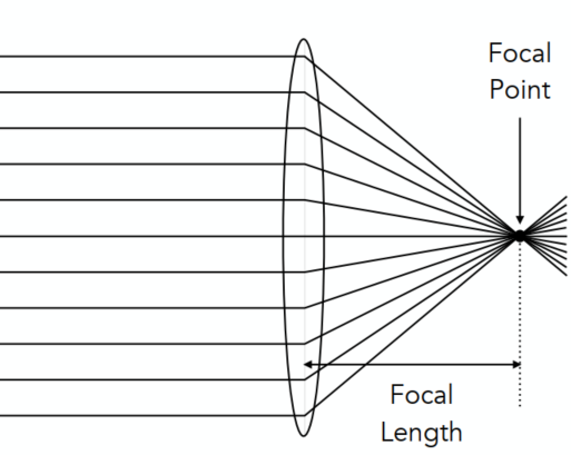
- All parallel rays entering a lens pass through its focal point
- All rays through a focal point will be in parallel after passing the lens
- Local length can be arbitrarily changed (actually in camera lens -> yes)
The Thin Lens Equation
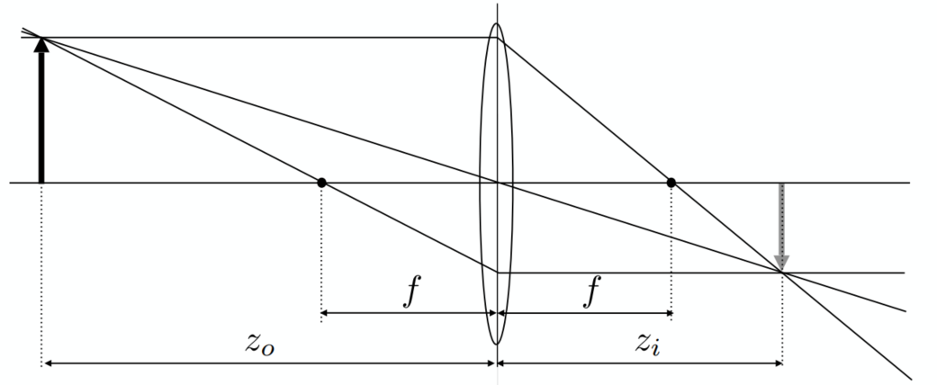
Gaussian Thin Lens Equation
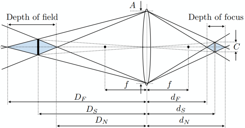
Defocus Blur
Computing Circle of Confusion (CoC) Size
If not at the focal plane -> not projected at the sensor plane -> blurry
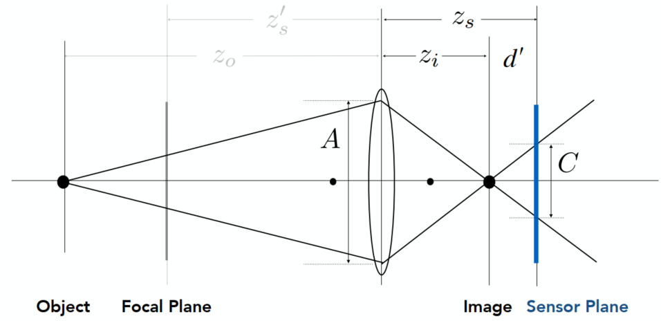
Circle of confusion is proportional to the size of the aperture
Ray Tracing for Defocus Blur (Thin Lenses)
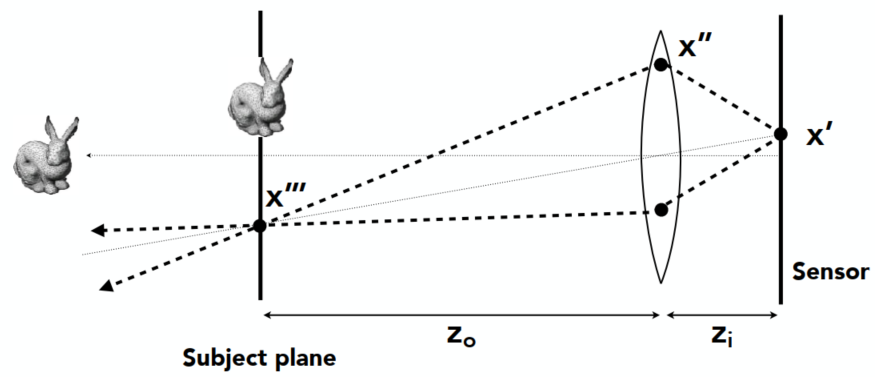
(One possible) Setup:
- Choose sensor size, lens focal length and aperture size
- Choose depth of subject of interest
- Calculate corresponding depth of sensor
Rendering:
- For each pixel
- Sample random points
- You know the ray passing through the lens will hit
- Estimate radiance on ray
Depth of Field
Circle of Confusion for Depth of Field
Depth range in a scene where the corresponding CoC is considered small enough
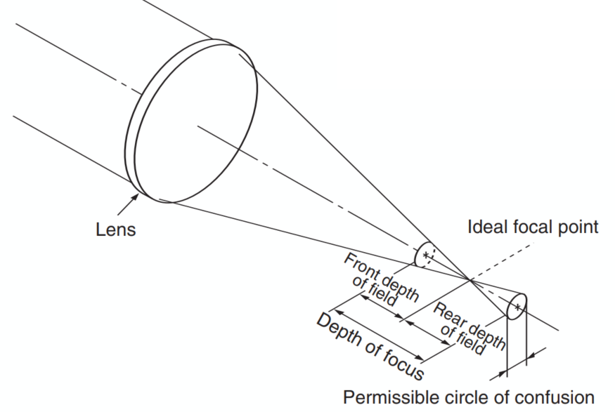
Depth of Field
Light Field / Lumigraph
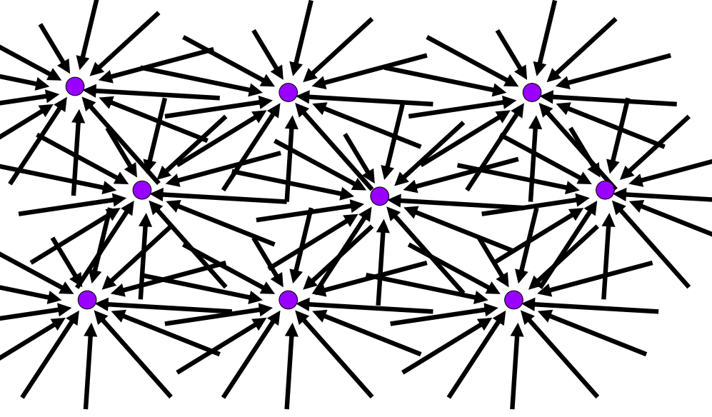
The Plenoptic Function
Function
The Plenoptic Function(全光函数) (Adelson & Bergen): The set of all things that we can ever see
Start with a stationary person and parameterize everything that can be seen
Grayscale Snapshot
The intensity of light
- Seen from a single view point
- At a singe time
- Averaged over the wavelengths of the visible spectrum
Color Snapshot
The intensity of light
A Movie
Add time:
Holographic Movie
Add location:
- Seen from any view point
- Over time
- As a function of wavelength
The Plenoptic Function (7 dimensions)
Can reconstruct every possible view, at every moment, from every position, at every wavelength
Contains every photograph, every movie, everything that anyone has ever seen (completely capture everything)
Sampling Plenotic Function (Top View)
Ray
Ignore the time and color at the moment: 5D (3D position + 2D direction)
Ray Reuse: Infinite line: assuming light is const (vacuum): 4D (2D pos + 2D dir, non-dispersive medium)
Only need plenoptic surface: The surface of a cube holds all the radiance info due to the enclosed obj
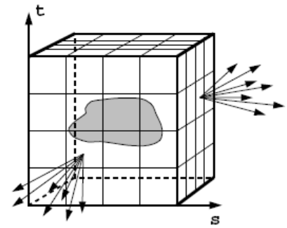
Lightfield: The intensity of light from any position to any direction (2D pos + 2D dir)
Synthesizing novel views
Lumigraph / Lightfield
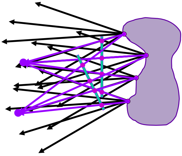
Outside convex space (The right side as a black box, and can be neglected. We only need to know what will be on the left side)

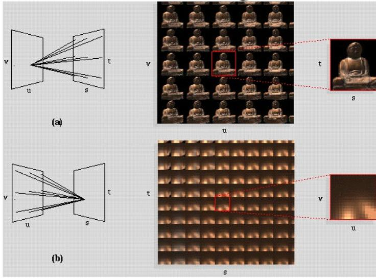
Organization: 2 planes (parameterization: uv and st) can define a lightfield
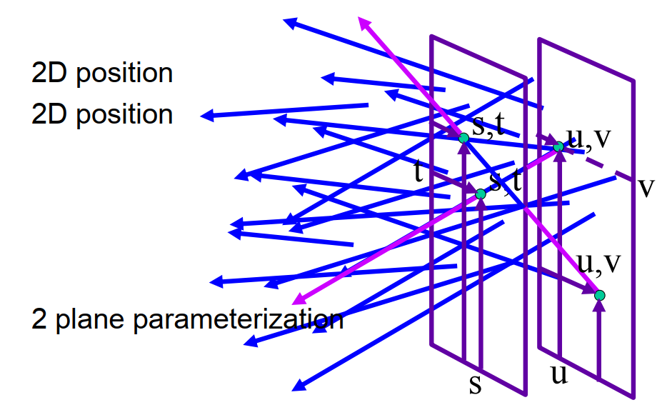
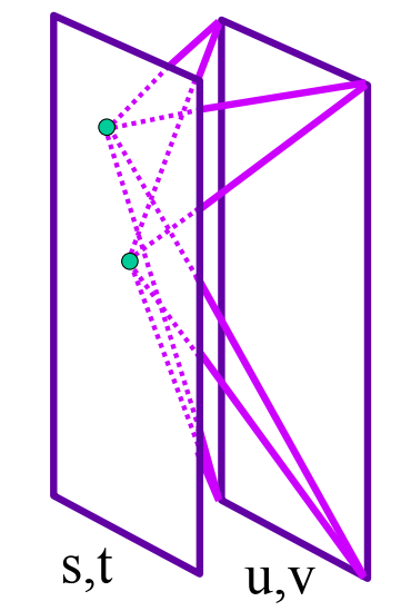
Hold st, vary uv => an image
Integral Imaging (“Fly’s Eye” Lenslets)
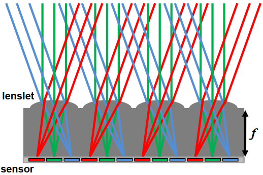
Spatially-multiplexed light field capture using lenslets: Impose fixed trade-off between spatial and angular resolution
Light Field Camera
[Ren Ng] Microlens design => Computational Refocusing (virtually changing focal length & aperture size, etc. after taking a photo)
Understanding
- Each pixel (irradiance) is now stored as a block of pixels (radiance) (The pixel is now the microlens)
- A close-up view of a picture taken
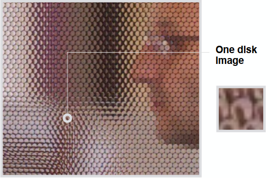
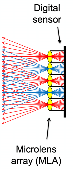
The left side of the microlens arrya is a light field
To Get a “Regular” Photo
- A simple case — always choose the pixel at the bottom of each block
- Then the central ones & the top ones
- Essentially “moving the camera around
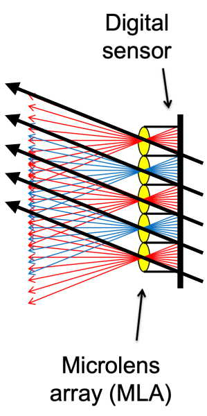
Computational Refocusing
- Same idea: visually changing focal length, picking the refocused ray directions accordingly
Properties
- The light field contains everything
Problem:
- Insufficient spatial resolution (same film used for both spatial and directional information)
- High cost (intricate designation of microlenses)
Computer Graphics is about trade-offs
Color and Perception (Lec. 20)
Physical Basis of Color
The Visible Spectrum of Light
Electromagnetic Radiation: Oscillations of different frequencies (wavelengths)
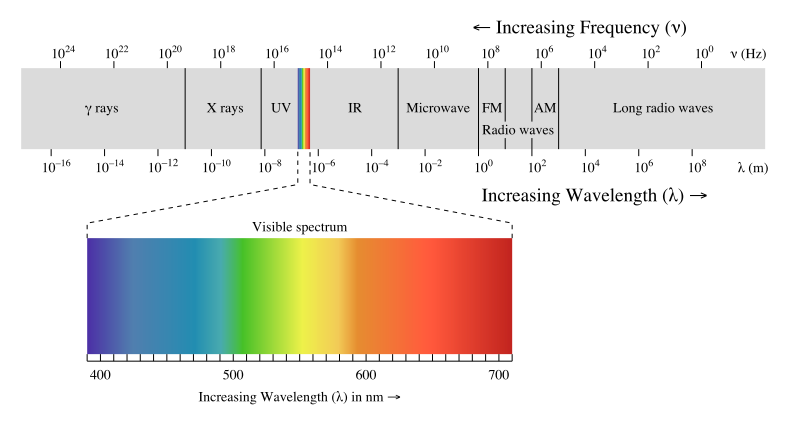
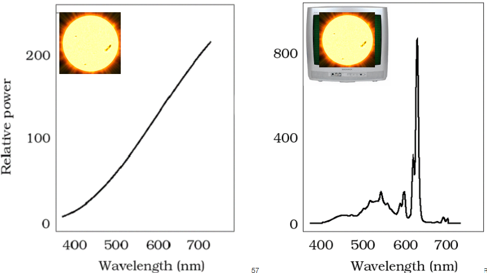
Spectral Power Distribution (SPD)
Salient property in measuring light: The amount of light present at each wavelength [radiometric units / nanometer OR unitless]
Daylight Spectral Power Distributions Vary
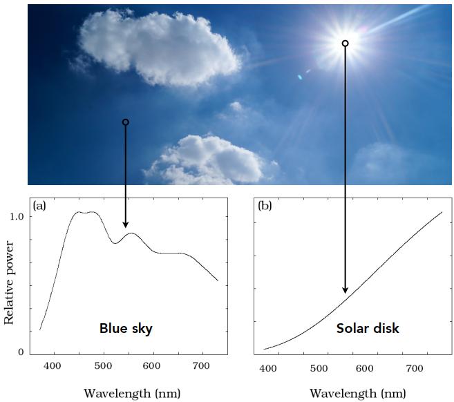
SPD is Linear: Different colors result in an addition of the wavelength distribution
Color
Color is a phenomenon of human perception (not a universal property of light)
Biological Basis of Color
Anatomy of The Human Eye
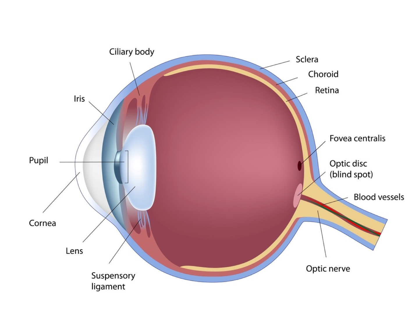
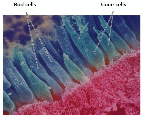
Retinal Photoreceptor Cells: Rods and Cones
Photoreceptor cells(感光细胞)
Rods: primary receptors in very low light (“scotopic” conditions) => more
Perceive only shades of grey, no color (the luminance)
Cones: primary receptors in typical light levels (“photopic”) => fewer
3 types (S/M/L) for different spectral sensitivity; Provide sensation of color
Spectral Response of Human Cone Cells
Three types: S, M, L (corres to peak response at low / medium / long wavelengths)
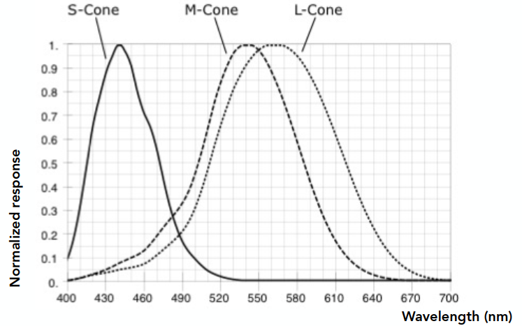
But the distributions of the 3 types of cone cells in different people are very different
Tristimulus Theory of Color
Spectral Respondse of Human Cone Cells
From the prev graph:
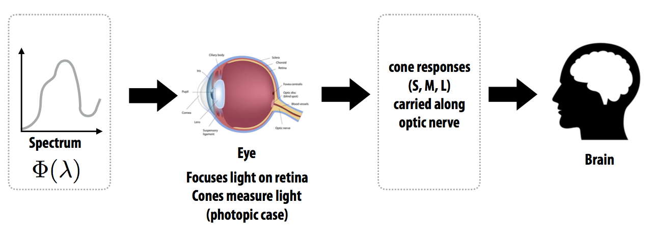
The Human Visual System
Human eye does not measure and brain does not receive info about each wavelength of light
=> The eye “sees” only 3 response values (S, M, L) and only info available to brain
Metamerism
Metamerism(同色异谱)
Metamers
Metamers are 2 different spectra (
Result: different spectra have the same color to a human
Critical to color reproduction: don’t have to reproduce the full spectrum of a real world scene
Metamerism
The theory behind color matching
Color Reproduction / Matching
Additive Color
- Given a set of primary lights, each with its own spectral distribution (e.g. R,G,B display pixels):
- Adjust the brightness of these lights and add them together:
- The color is now described by the scalar values:
Addition: when RGB are all 255, get the color of white
Additive color matching experiment: Use primary colors to obtain a required color => may result in negative values
CIE RGB Color Matching
Same as before but primaries are monochromatic light (single wavelength) and the test light is also a monochromatic light
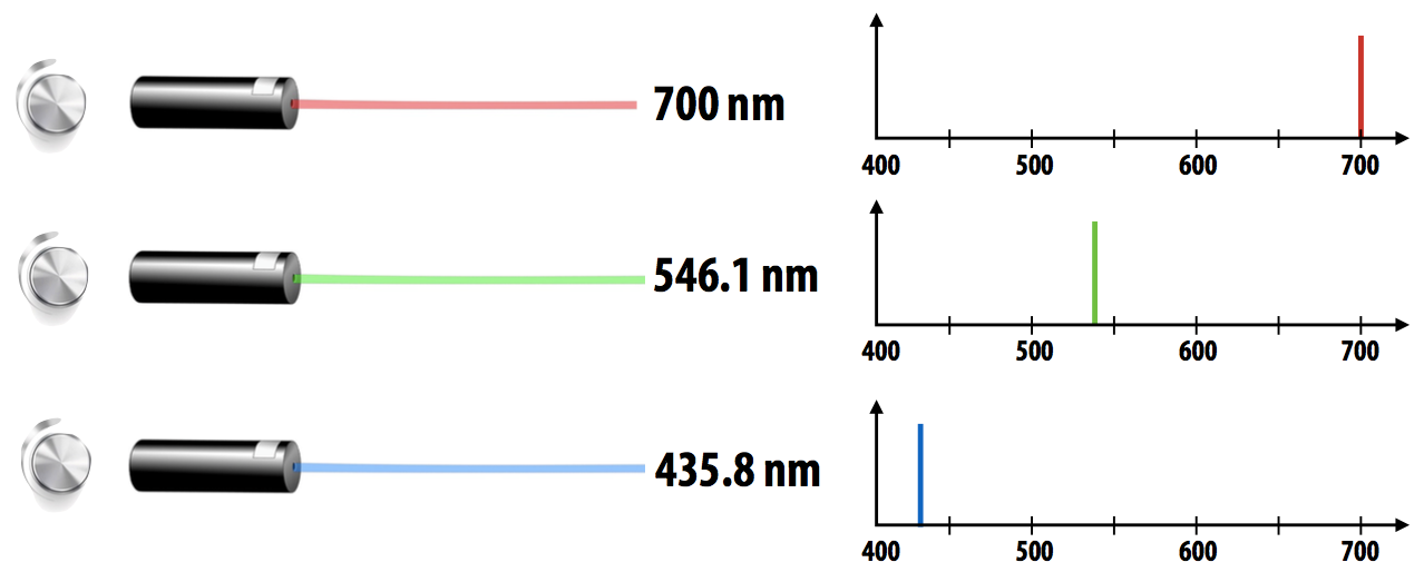
Function: Graph plots how much of each CIE RGB primary light must be combined to match a monochromatic light of wavelength given on x-axis
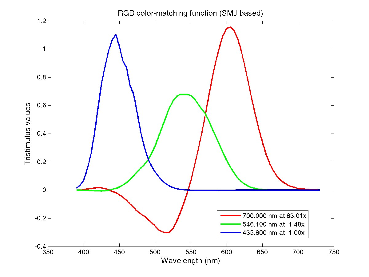
For any given color, it can be represented by these functions
Color Space
Standard Color Space
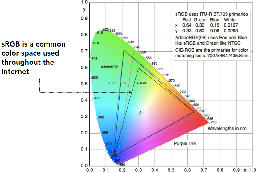
Standardized RGB (sRGB)
- Make a particular monitor RGB standard
- Other color devices simulate that monitor by calibration
- Widely adopted today (most monitors are sRGB)
- Gamut(色域) is limited
A Universal Color Space: CIE XYZ
Imaginary set of standard color primaries X, Y, Z (artifically defined, red has no negative values)
- Primary colors with these matching functions do not exist
- Y is luminance (brightness regardless of color)
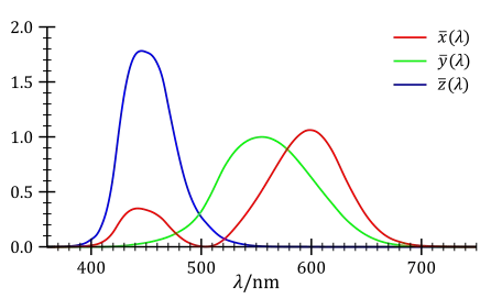
Designed such that:
- Matching functions are strictly positive
- Span all observable colors
Separating Luminance, Chromaticity
Luminance: Y
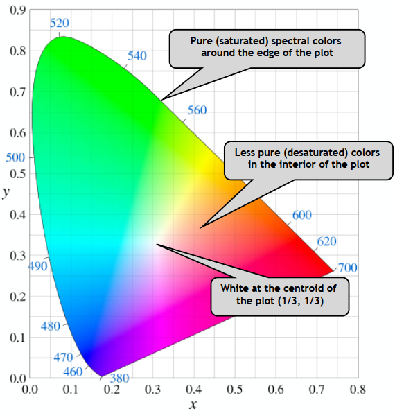
Chromaticity: x, y, z, defined as: (
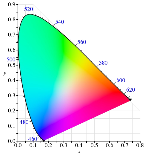
CIE Chromaticity Diagram
The diagram represents the Gamut
The curved boundary:
- Named spectral locus
- Corresponds to monochromatic light (each point represnting a pure color of a single wavelength)
Any color inside is less pure (mixed, white is the least pure color)
Gamut
Gamut is the set of chromaticities generated by a set of color primaries. Different color spaces represent different ranges of colors, so they have different gamuts (cover different regions on the chromaticity diagram).
Perceptually Organized Color Spaces
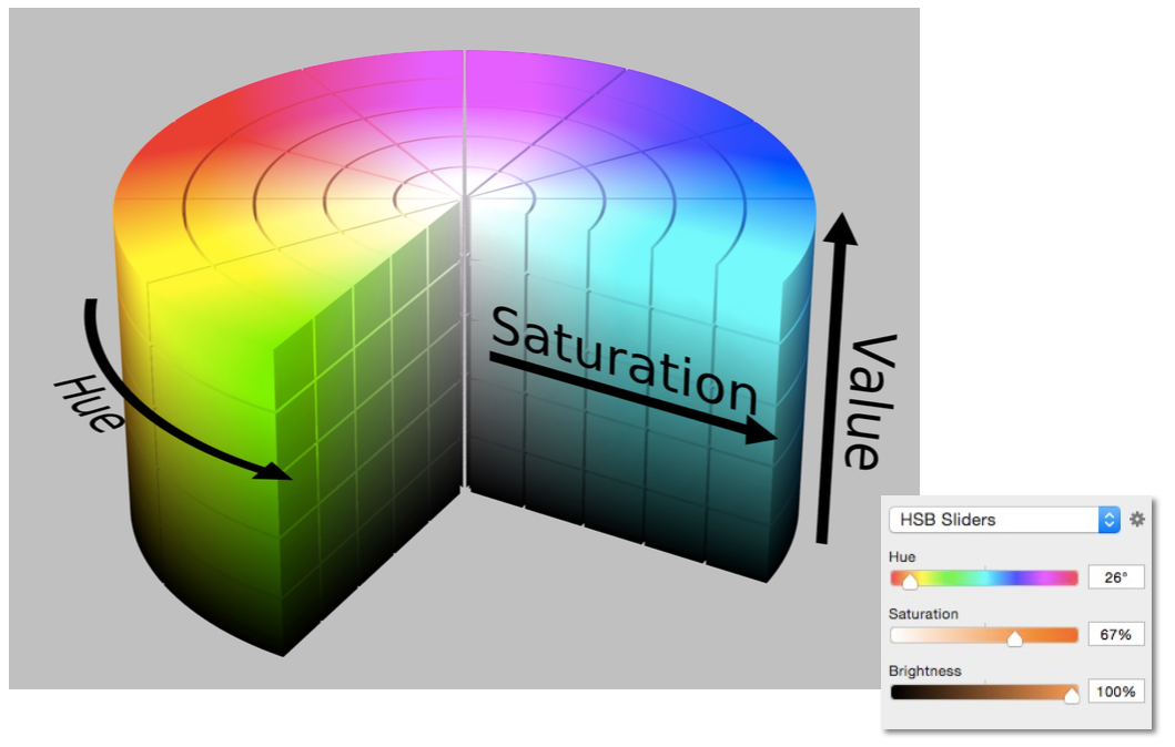
HSV Color Space (Hue-Saturation-Value)
Axes correspond to artistic characteristics of color
Widely used in a “color picker” (e.g., in Photoshop)
In color adjustment: HSL (Hue-Saturation-Lighness)
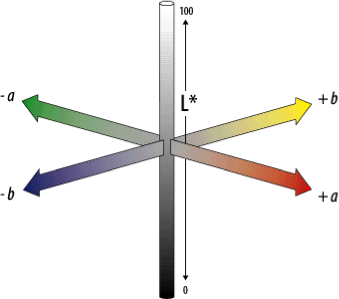
CIELAB Space (AKA L*a*b)
A commonly used color space that strives for perceptual uniformity
L* is lightness (brightness)
a* and b* are color-opponent pairs
- a* is red-green
- b* is blue-yellow
Opponent Color Theory
There’s a good neurological basis for the color space dimensions in CIELAB
The brain seems to encode color early on using three axes:
- white — black, red — green, yellow — blue
The white — black axis is lightness; the others determine hue and saturation
And colors / lightness are relative
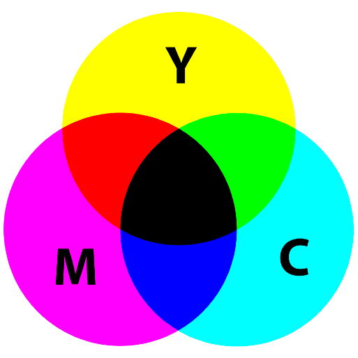
CMYK: A Subtractive Color Space
CMYK: Cyan, Magenta, Yellow, and Key (Black) (for key: though it can be obtained by mixing, but lower the costs in printing)
The more we mix, the darker it will be.
Animation (Lec. 21-22)
-> See more in GAMES103 - Physics-Based Animation